

Sequence evaluation
When processing sequences obtained from a vendor, it is useful to have an idea of how well the sequencing reactions worked, both in an absolute sense and relative to other recently obtained sequences in the same project. What follows is a primary sequence independent method of evaluating a collection (i.e. and order from an outside vendor) of sequences.
The first step is to align sequences by nucleotide index (ignoring the actual sequence). Start by reading the sequences into a list. I use the list s.b to hold forward (5’ to 3’) sequences, and the list s.f to hold the reverse (but in the 5’ to 3’ orientation, as sequenced) sequences:
1 | rm(list=ls(all=TRUE)) |
Next determine the number of files read and create a list of that length to hold the sequences. Then read them in and inspect a sequence:
1 | s.b <- list() |
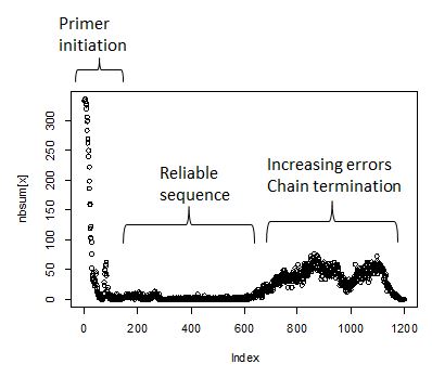
Note that ambiguities are indicated with an “n”. The sequence evaluation will involve counting the number of ambiguitites at each index position. The expectation is that initially - first 25 or so bases - will have a large number of ambiguities, falling to near zero at position 50. This is the run length required to get the primer annealed and incoporating nucleotides. Next will follow 800-1200 positions with near zero ambiguity count. How long exactly is a function of the sequencing quality. Towards the end of the run the ambiguities begin to rise as the polymerase loses energy. Finally the ambiguity count will fall as the reads terminate.
Create a vector nbsum that will tally the count of ambiguities at a given index. Then process through each sequence and count, at each index, the number of ambiguities. The total count of ambiguities is entered into nbsum at the corresponding index position.
1 | for( i in 1:length(s.b)){ |
Overlay the reverse reads in red.
1 | nfsum <- vector( mode="integer", length=2000) |

I have created a shiny app that implements the above code. Download it here.

Automated colony counting
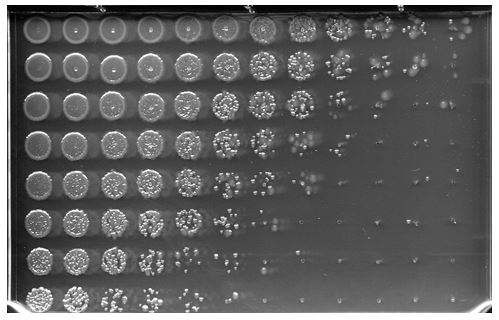
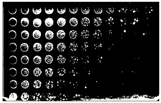
In a previous post I discussed using a 96 channel pipettor and Omniplates for titering bacterial cultures. Here I show how to automate the counting process. Start with a two dimension serial dilution of a culture as shown on the plate below:
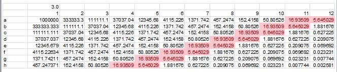
A 2D dilution simulation suggests that a small number of regions will be in the correct range for accurate titer determination (red cells):
Capture an image:
1 | rm(list=ls(all=TRUE)) |
and convert to binary black/white:
1 |
|

Next perform a series of erodes and dilates to sharpen the colonies:
1 |
|

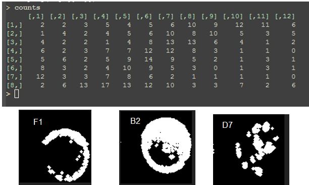
Then count. I will decompose the main image into 96 smaller images which can then each be processed individually. Identify the upper right corner origin and the segment.width, 103 pixels in this case. Print out the coordinates of individual segments
1 | segment.width <- 103 |

Now count the spots in the individual images algorithmically and also manually for those wells that can be counted. Plot and compare.
1 | #reorder by column |
The diagonal with a majority of counts >10 would be predicted to give the most reliable results.
Now compare algorithmic vs. manually determined counts:
1 | names(d)[2:3] <- c("algorithm","manual") |
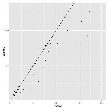
Make an attemp to fit a couple of polynomial lines - for predictive purposes.
1 |
|

Looks like not much advantage to the polynomial fit so I will fit a line and extrapolate.
Print out algorithmically determined counts, predicted (i.e. manually determined) counts, and the difference.
1 |
|

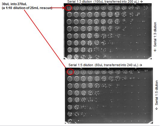
High throughput titering
Plating colonies on 10cm dishes, either for titering or for isolating clones, is a resource intensive process. Eliminate some of the tedium and expense by reducing the scale. Serial dilutions are performed in a 96 well plate filled with bacterial growth media e.g. 270uL per well, transferring 30uL down the columns for a 1:10 dilution per row. Next, using a 96 channel Biomek NX, 10uL of dilute bacteria from each well are deposited on the surface of an Omni plate filled with 60mL LB agar + AMP at 100ug/mL. Dilute such that counts are in the range of 5 to 20 per spot.
Nunc cat# 267060
Nunc cat# 242811 OmniTray Single Well w/lid 86x128mm (pictured below)

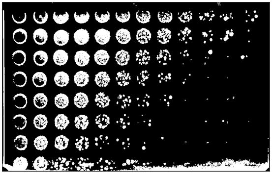
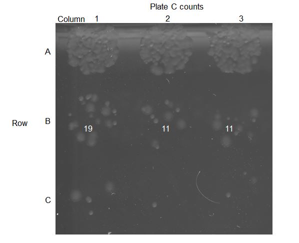
A single Omniplate can substitute for 96 10cm dishes, though in practice many of the Omniplate regions will not be countable. Below are some images of colony growth on the first three rows of an Omni plate.

Close up of 9 regions, with counts indicated in white:
Comparison of counts from a 10cm dish to counts from an Omniplate. Expected counts are an estimate based on OD600.
OD600 estimate is >100 fold off.

Calculated titers. Note that results are more consistent with the wells containing a higher number of counts - Row B:

Referencer
A couple of options for free, web based bibliography managers are Mendeley and Zotero. Given that Mendeley is owned by Elsevier, they are not an option. I started with Zotero, some configuration elements I will outline below, but eventually dropped them for Referencer. I like the idea of having complete control over my library. I am not interested in the “social” features of Zotero, I found upgrades to be difficult, and didn’t like the file structure utilized. Referencer is extremely simple, easy to install and configure, and gets the job done. I don’t anticipate many “upgrades” to the Referencer software - hopefully it will be maintained well into the future. I replicate the files to a cloud server for easy backup.
Referencer
#apt-get install referencer
Zotero
do not export, backup the database directory to retain metadata
~/.zotero/zotero/<3xdb….>/zotero…
the “pipes” subdir will not copy, be sure to compensate
pacman -S alsa-lib dbus-glib gcc-libs
pacman -S gtk2 nss #these were already installed
To configure the Zotero webdav server on Hostgator:
www.mysite.com/owncloud/remote.php/webdav ( /zotero automatically appended)
you will be prompted to create directory
Associate GPS coordinates with a street address
Obtain street addresses
We would like to associate trees with street addresses when possible. When collecting tree data, we could also make note of the nearest address. Since we are collecting longitude/latitude data anyway, it would be convenient if we had a list of street addresses with associated longitude/latitude. This would allow us to auto-populate an address field based on longitude/latitude data. How does one obtain a list of all street addresses in town with longitude/latitude data? Let’s start with obtaining addresses alone. Addresses are availble commercially e.g. from the post office, but for a substantial fee. Since this is a volunteer effort, I want to see what I can get for free. Our town publishes property assessments on a regular basis, but this is hardcopy in the local paper. Though assessments are available online, it is through a query interface providing one at a time, with no obvious way to download the entire list. I was able to find our town’s street sweeping schedule which supplies a list of all streets in html format:
etc.
Copy paste into a text editor and with a little manipulation in R, I can get a vector of street names:
1 | > rm(list=ls(all=TRUE)) |
Looks like about 561 streets total. From my hardcopy assessment I learn that:
- Most streets don’t begin with 1 as the first address
- Addresses aren’t consecutive - there can be many gaps in numbering
- Most streets have fewer than 200 addresses
- A few of the main streets have up to 1600 addresses
Query for GPS coordinates
To obtain street addresses with lng/lat data I will use the DataScienceToolkit Google Style geocoder. To obtain coordinates I need to submit an address that looks like:
1 Aberdeen Road, Arlington, MA
This will return a data set that looks like:
[{“geometry”:{“viewport”:{“northeast”:{“lng”:-71.188745,”lat”:42.424604},”southwest”:{“lng”:-71.190745,”lat”:42.422604}},”location_type”:”ROOFTOP”,”location”:{“lng”:-71.189745,”lat”:42.423604}},”types”:[“street_address”],”address_components”:[{“types”:[“street_number”],”short_name”:”1”,”long_name”:”1”},{“types”:[“route”],”short_name”:”Aberdeen Rd”,”long_name”:”Aberdeen Rd”},{“types”:[“locality”,”political”],”short_name”:”Arlington”,”long_name”:”Arlington”},{“types”:[“administrative_area_level_1”,”political”],”short_name”:”MA”,”long_name”:”MA”},{“types”:[“country”,”political”],”short_name”:”US”,”long_name”:”United States”}],”formatted_address”:”1 Aberdeen Road Arlington MA”}]
You can see that lng= -71.188745 and lat=42.424604. I want to submit algorithmically, using a post to their URL. The post will look like:
I also want to count up the street addresses beginning at 1. This will give me a lng/lat for every address depending on how the geocoder handles addresses that don’t exist. Let’s find out.
1 | > |
Allen Street addresses begin at 12 so it looks like we will assigned lng/lat to nonexisting addresses. 1 and 2 share the same lng/lat. This also happens at the high end e.g. if the highest address is 100, 1 through 100 will be assigned unique lng/lats, and then the lng/lats become constant. Modify the code to stop querying once both lng and lat aren't changing.
BU 353 USB GPS unit
Handling GPS data
Hardware
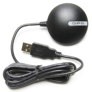
Be sure to purchase a unit that will broadcast NMEA compliant sentences. I chose the Globalsat BU-353 shown below. This is a USB device that obtains power through the USB, but also has an internal battery for short term memory. Plug the unit into your laptop and allow a few minutes to get a fix. The led will start blinking once a fix has been obtained. You will not need any of the software provided with the unit.
Software
Guile 1.8 a dialect of Scheme/Lisp
gpsd a gps daemon. You will want to install the software compiled for your system, e.g. on Arch use
>pacman -S gpsd gpsd-clients
Direct access to tty
By default your gps unit is assigned to /dev/ttyUSB0, but you should check to make sure:
>dmesg | grep -i USB
[11250.384023] usb 4-2: new full-speed USB device number 2 using uhci_hcd
[11250.669968] usbcore: registered new interface driver usbserial
[11250.669991] USB Serial support registered for generic
[11250.670030] usbcore: registered new interface driver usbserial_generic
[11250.670033] usbserial: USB Serial Driver core
[11250.673280] USB Serial support registered for pl2303
[11250.685151] usb 4-2: pl2303 converter now attached to ttyUSB0
[11250.685174] usbcore: registered new interface driver pl2303
[11250.685177] pl2303: Prolific PL2303 USB to serial adaptor driver
Set access, change the baud rate and put the GPS in NMEA mode. Look at some of the output:
>sudo chmod 666 /dev/ttyUSB0 && stty -F /dev/ttyUSB0 ispeed 4800
>cat /dev/ttyUSB0
$GPGSA,A,3,15,14,09,18,21,24,22,06,19,,,,1.9,1.2,1.4*36
$GPGSV,3,1,12,18,71,317,34,24,63,112,31,21,52,212,28,15,42,058,34*71
$GPGSV,3,2,12,22,37,301,28,14,21,250,24,09,07,035,21,19,06,316,13*73
$GPGSV,3,3,12,06,05,279,18,26,01,060,,03,01,294,,28,01,024,*7F
$GPRMC,224355.000,A,1825.0332,N,02111.3093,W,0.13,134.34,050513,,,A*75
$GPGGA,224532.000,1825.0301,N,02111.3093,W,1,08,1.3,39.8,M,-73.7,M,,0000*25
$GPGSA,A,3,15,14,09,18,21,24,22,06,19,,,,1.9,1.2,1.4*36
$GPRMC,224356.000,A,4225.0330,N,02111.3093,W,0.33,145.51,050513,,,A*73
$GPGGA,224357.000,1825.0328,N,07111.3092,W,1,09,1.2,81.8,M,-33.7,M,,0000*5F
$GPGSA,A,3,15,14,09,18,21,24,22,06,19,,,,1.9,1.2,1.4*36
$GPRMC,224357.000,A,1825.0328,N,02111.3092,W,0.28,151.99,050513,,,A*71
Use Ctrl-C to stop the process.
Pick a sentence format that contains the coordinate information you wish to extract. I chose GPGGA.
>cat /dev/ttyUSB0 | grep GPGGA
$GPGGA,124532.000,1825.0301,N,02111.3093,W,1,08,1.3,39.8,M,-73.7,M,,0000*25
$GPGGA,124532.000,1825.0301,N,02111.3093,W,1,08,1.3,39.8,M,-73.7,M,,0000*25
$GPGGA,124532.000,1825.0301,N,02111.3093,W,1,08,1.3,39.8,M,-73.7,M,,0000*25
$GPGGA,124532.000,1825.0301,N,02111.3093,W,1,08,1.3,39.8,M,-73.7,M,,0000*25
$GPGGA,124532.000,1825.0301,N,02111.3093,W,1,08,1.3,39.8,M,-73.7,M,,0000*25
$GPGGA,124532.000,1825.0301,N,02111.3093,W,1,08,1.3,39.8,M,-73.7,M,,0000*25
$GPGGA,124532.000,1825.0301,N,02111.3093,W,1,08,1.3,39.8,M,-73.7,M,,0000*25
$GPGGA,124532.000,1825.0301,N,02111.3093,W,1,08,1.3,39.8,M,-73.7,M,,0000*25
$GPGGA,124532.000,1825.0301,N,02111.3093,W,1,08,1.3,39.8,M,-73.7,M,,0000*25
$GPGGA,124532.000,1825.0301,N,02111.3093,W,1,08,1.3,39.8,M,-73.7,M,,0000*25
You can extract to a text file using:
cat /dev/ttyUSB0 | grep --line-buffered GPGGA > output.txt
Now with further munging you can extract the coordinates. I’ll save that for the next section where I use gpsd.
Using gpsd
Plug in your gps unit and start up gpsd. You will need to know the tty to which it is connected, see above.
gpsd -b /dev/ttyUSB0
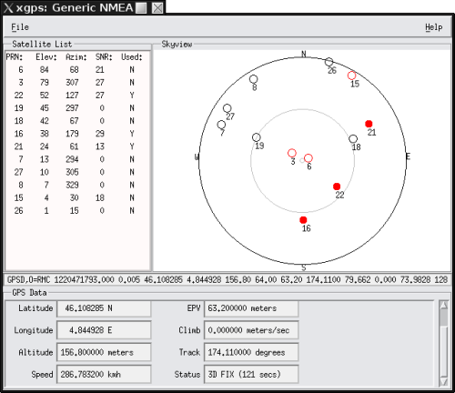
This launches the daemon which is now ready to be configured to accept requests. The “-b” switch means read only, to prevent writing that may lock up the unit. Use at your discretion. To verify the daemon is broadcasting, you can run either xgps (gui) or cgps, gpsmon (text) if you installed the client tools.
>gpsmon
If everything is working you should see your coordinates displayed in the interface. Here is an example of what the xgps interface looks like:
Next we want to algorithmically extract coordinates from the daemon. Here I am using Guile. First I import two modules, rdelim which provides the read-line method, and srfi-1 which allows me to extract elements of a list using first, second, third, etc. Create a socket, connect the socket to port 2947 on my local machine and send the message "?WATCH={\"enable\":true,\"nmea\":true}" to indicate I am waiting for NMEA sentences.
(use-modules (ice-9 rdelim))
(use-modules (srfi srfi-1))

(define coords '())

(let ((s (socket PF_INET SOCK_STREAM 0)))
     (connect s AF_INET (inet-pton AF_INET "127.0.0.1") 2947)
     (send s "?WATCH={\"enable\":true,\"nmea\":true}")
     (do ((line  (read-line s) (read-line s)))
         ((string= (substring line 1 6) "GPGGA")
         (set! coords (list (third (string-split line #\,)) (fourth (string-split line #\,)) (fifth (string-split line #\,)) (sixth (string-split line #\,)))))))
I keep resetting the variable ‘line’ until I find a line that starts with GPGGA. Once obtained, I extract the coordinates and form a list which is named ‘coords’. Run the method to get the ouput below.
guile> guile> guile> guile> guile> ("4225.0384" "N" "78411.3104" "E")
guile>
You now have a list of coordinates which can now be converted into the desired format.
Linux Distributions
I have used three Linux distributions: Ubuntu, Arch, and Debian. Here are my thoughts on the strengths and weaknesses of each.
Ubuntu
For a newcomer to Linux, Ubuntu is a natural choice. Canonical, the company behind Ubuntu, is a business, and as a business it is in their best interest to make Linux installation a no brainer. All drivers are included in the image and a live CD will allow you to experience Ubuntu without even installing the software. This allows you to determine if the distribution will work with your hardware, and test drive some of the applications. Once installed you will find all the features you expect from a mature desktop operating system. With a large user base, someone has probably already found a fix to problems you may experience.
Users migrating to Linux, myself included, are often migrating for the purpose of privacy and control. I don’t want to pay $1000 for a computer and then have to get Microsoft’s permission to use it. Meanwhile every keystroke is logged and my search queries a catalogued at headquarters. By signing up with Ubuntu, you are in for a similar experience. Desktop search pipes your queries to Amazon and the Ubuntu software manager will annoy you with advertisements for non-free crapware. Once you have become comfortable with Linux using Ubuntu, it is time to move on.
Arch
I thought I wanted a minimalist system, so I committed to Arch and the I3 window manager. Arch is a great system for someone who wants to learn Linux inside out. Nothing is preconfigured, forcing you to learn the intricasies of the configuration files. Most users will be hard core programmers - you have to be to deal with installation and configuration - so all problems have been encountered and solutions explicitly provided. I never had an Arch problem I couldn’t solve from reading the wiki. One quirk (feature?) of Arch is the rolling releases. When installing packages, you almost always need to run a system upgrade. 99% of the time this completes without problems, but occasionally, for example 2013-06-03 the file system directory layout was changed and a significant effort had to be invested in completing the upgrade. “Always read the Arch news before upgrading” - Arch is thoroughly and expertly documented, but this requires religious devotion.
The problem with Arch is that it requires a lot of work and time. Everything needs to be configured. For example, if you plug in a USB stick, nothing happens unless you configured auto-mount. I quickly came to realize that I don’t want to be a Linux guru, I just want to use Linux to get things done. That is what led me to Debian.
Debian
Debian is the distribution on which many other distributions (including Ubuntu) are built. Debian has the reputation for stability, with major releases occurring about every 2 years. Releases make use of well tested applications, sometimes a version or two behind what is currently available, to guarantee stability. Debian’s package manager is field tested and shared by many other distributions. Most software written for Linux will have an installation package for Debian. As I usually buy older computers with less memory, I use the minimalist Xfce window manager. Xfce has a clean layout, doesn’t install a lot of unnecessary software, yet provides the essentials you would expect in a modern window manager. There is a Debian installer that defaults to using Xfce as the window manager. I have been using Debian for a couple of years now and can report that I have encountered no issues that would prevent the average user from switching from Windows or Apple to Linux. The one exception would be Microsoft Office file compatibility. LibreOffice does a good job, but complex documents may not render properly.
Population Genetics Chpt 5 End
Chapter 5 End Problems
Problem 2
1 | condition <- letters[1:4] |

Shifting balance favors smaller N and smaller m so C is the favored condition.
Problem 6
Start by setting r = x/ny to get the break even n. Anything larger is needed for altruistic behaviour to be favored by kin selection.
0.25 = 0.4/0.2n or n=0.4/(0.2*0.25) = 8 or greater
Problem 11
1 | area <- c("dark","dark","light","light") |
Problem 14
1 | J.1 <- c(0.12, 0.8, 0.06, 0.02) |
Problem 15
1 | J.1 <- c(0.3, 0.5) |