Automated colony counting

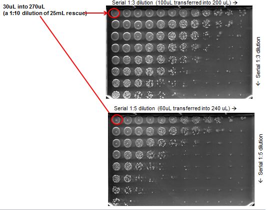
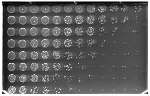
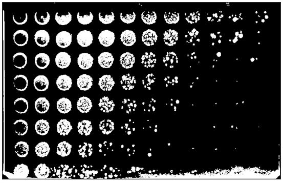
In a previous post I discussed using a 96 channel pipettor and Omniplates for titering bacterial cultures. Here I show how to automate the counting process. Start with a two dimension serial dilution of a culture as shown on the plate below:

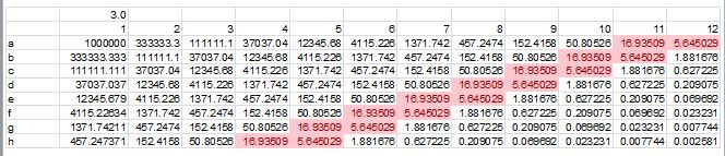
A 2D dilution simulation suggests that a small number of regions will be in the correct range for accurate titer determination (red cells):

Capture an image:

1
2
3
4
5
6
7
8
9
10
rm(list=ls(all=TRUE))
library(ggplot2)
library("EBImage")

file.prefix <- "3c"
f<- paste( getwd(), "/input/", file.prefix, ".JPG", sep="")

pic = readImage(f)
display(pic)

and convert to binary black/white:

1
2
3
4

pic.thresh <- pic > 0.4
#display(pic.thresh)

Next perform a series of erodes and dilates to sharpen the colonies:

1
2
3
4
5

pic2 <- erode(pic.thresh)
pic2 <- dilate(pic2)
display(pic2)

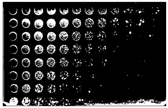
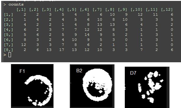
Then count. I will decompose the main image into 96 smaller images which can then each be processed individually. Identify the upper right corner origin and the segment.width, 103 pixels in this case. Print out the coordinates of individual segments

1
2
3
4
5
6
7
8
9
10
11
12
13
14
15
16
17
18
19
20
21
22
23
24
25
26
27
28
29
30
31
32
33
34
35
segment.width <- 103
origin <- c(35,20)

# A[ rows, cols ]
imgs <- rep(list(matrix(data=NA,nrow=segment.width+1,ncol=segment.width+1)), 96)

counts <- rep(NA, 96)

k <- 1
for(i in 1:8){
for(j in 1:12)
{
cat( "pic2[",(origin[1] + 1 + (j-1)*segment.width),":",(origin[1]+ (j)*segment.width )," , ")
cat( (origin[2]+ (i-1)*segment.width),":",(origin[2]+ (i)*segment.width ),"]\n")

imgs[[k]] <- imageData( pic2 )[ (origin[1] + 1 + (j-1)*segment.width):(origin[1]+ (j)*segment.width ),
(origin[2]+ (i-1)*segment.width):(origin[2]+ (i)*segment.width ) ]
img.label <- bwlabel(imgs[[k]])
counts[k] <- max(img.label)
k <- k+1
rm(img.label)
}
}

pic2[ 139 : 241 , 20 : 123 ]
pic2[ 242 : 344 , 20 : 123 ]
pic2[ 345 : 447 , 20 : 123 ]
pic2[ 448 : 550 , 20 : 123 ]
...

#display a segment

display(imgs[[77]])


Now count the spots in the individual images algorithmically and also manually for those wells that can be counted. Plot and compare.

1
2
3
4
5
6
7
8
9
10
11
12
13
14
15
16
17
18
19
20
21
22
23
24
25
26
27
28
29
#reorder by column
counts.m <- matrix(counts, nrow=8, byrow=TRUE)
counts.bycol <- as.vector(counts.m)

#convert a well number to row/column designation.
getWell96 <- function( id ){
n <- 1:96
row <- rep(LETTERS[1:8],12)
col <- sort(rep(1:12, 8))
name <- I(paste(row,col, sep="")) #I() is as.is to prevent factorization
well.ids <- data.frame(name, n)

if( id %in% name) {well.ids[well.ids$name==id,"n"]
}else{
well.ids[well.ids$n==id,"name"]}
}

wells <- sapply( 1:96 , getWell96)
manual <- NA #to hold manual counts

results <- data.frame(wells, counts.bycol, manual)

#count a bunch manually
results[ results$well=="A10","manual"] <- 16
results[ results$well=="A11","manual"] <-11
results[ results$well=="A12","manual"] <-8
results[ results$well=="B9","manual"] <-13
...

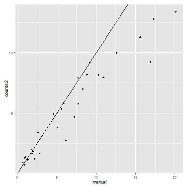
The diagonal with a majority of counts >10 would be predicted to give the most reliable results.
Now compare algorithmic vs. manually determined counts:

1
2
3
4
5
6
7
names(d)[2:3] <- c("algorithm","manual")

x <- d$algorithm
y <- d$manual
#we will make y the response variable and x the predictor
#the response variable is usually on the y-axis
plot(x,y,pch=19)

Make an attemp to fit a couple of polynomial lines - for predictive purposes.

1
2
3
4
5
6
7
8
9
10
11
12
13
14
15
16
17
18

#fit first degree polynomial equation:
fit <- lm(y~x)
#second degree
fit2 <- lm(y~poly(x,2,raw=TRUE))
fit3 <- lm(y~poly(x,3,raw=TRUE))

xx <- seq( 1,25, length=50)
plot(x,y,pch=19, ylim=c(0,15), xlim=c(0,15))
lines(xx, predict(fit, data.frame(x=xx)), col="red")
lines(xx, predict(fit2, data.frame(x=xx)), col="blue")
#lines(xx, predict(fit3, data.frame(x=xx)), col="green")

abline(0,1)

#y = 1.00008x -0.018513x^2 - 0.137933
b <- fit[[1]][1]
m <- fit[[1]][2]

Looks like not much advantage to the polynomial fit so I will fit a line and extrapolate.

Print out algorithmically determined counts, predicted (i.e. manually determined) counts, and the difference.

1
2
3
4
5
6
7
8
9

results$predicted <- round( predict(fit, data.frame(x=results$counts.bycol)), digits = 0)
results$delta <- results$predicted - results$counts.bycol
predicted <- matrix(results$predicted, nrow=8, byrow=FALSE)

counts.m
predicted
predicted - counts.m

Share