eStudio is a Java applet that runs in a browser. eStudio can be used to display a continuous loop of images on any computer with a browser. The features of eStudio are:
Display a continuous cycle of images. Image number is limited by available RAM
Images are grouped by categories, one category per subdirectory
Customize to use your own images
Optional annotation can be displayed with the image
Working example provided
Turn a laptop into a "kiosk" style display
Runs in any browser equipped with Java 1.4 or higher plug-in
Currently works on Windows only
Installation
Create an installation directory on your hard drive.
Download eStudio.zip into the installation directory. Unzip
Click on start.html to launch the applet.
Click on customize.html for customization information.
#Calculate each summary statistic using dplyr's group_by function
Sp <-(group_by(d, subpop)%>% summarize(sum(p)))[,2]#sum of p within subpopulation n <-(group_by(d, subpop)%>% summarize(length(p)))[,2]#count p.bar <-(group_by(d, subpop)%>% summarize(mean(p)))[,2]#mean p Sp2 <-(group_by(d, subpop)%>% summarize(sum(p2)))[,2]#sum p squared
H.bar <-(group_by(d, subpop)%>% summarize(mean(H)))[,2]#mean H d2 <- data.frame(c(Sp, n, p.bar, H.bar, Sp2)) names(d2)<-c("Sp","n","p.bar","H.bar","Sp2") np.bar2 <- d2$n*d2$p.bar^2
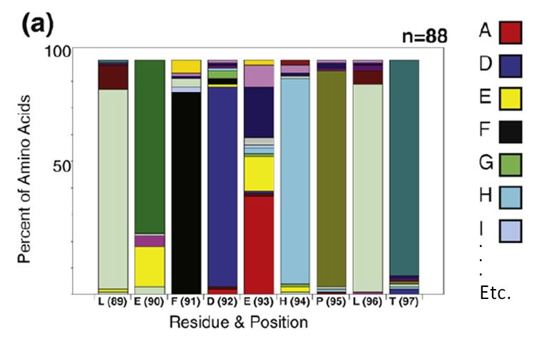
After perfoming error prone PCR (random) or oligonucleotide (directed) mutagenesis you will want to visualize your sequences and determine the rate of mutation incorporation. A typical visualization is the stacked bar chart as in this figure from Finlay et al. JMB (2009) 388, 541-558:
To decode this graphic you must:
estimate the percentage of each amino acid by comparison to the Y axis
compare relative amino acid abundance by comparing the area of boxes
correlate color with amino acid identity
compare to the reference sequence at the bottom of the graph
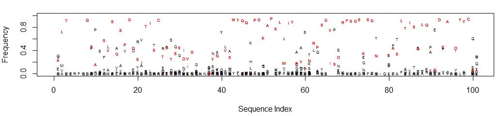
An easier to interpret graphic would be a scatter plot of sequence index (i.e. nucleotide position) on the X axis vs frequency on the Y. The data points are the single letter amino acid code. Highlight the reference sequence with a red letter.
The first step is to align all sequences. Start with a multi-fasta file of all sequences:
Above I have labeled my parental reference sequence “ref”. Use clustalo to perform the alignment and request the output in “clustal” format. The clustalo command can be run from within R using the system command. Read the alignment file into a matrix:
At each position determine the frequency of all 20 amino acids. Set up a second matrix that has one dimension as the length of the sequence and the other as 20 for each amino acid. This is the matrix that will hold the amino acid frequencies.
The R package “seqinr” provides a constant containing all single character amino acids as well as asterisk for the stop codon. Use this to name the rows of the frequency matrix.
library(seqinr)
levels(SEQINR.UTIL$CODON.AA$L)
[1] "*" "A" "C" "D" "E" "F" "G" "H" "I" "K" "L" "M" "N" "P" "Q" "R" "S" "T" "V"
[20] "W" "Y"
aas <- c(levels(SEQINR.UTIL$CODON.AA$L), 'X')
freqs <- matrix( ncol=dim(seqs.aln)[2], nrow=length(aas))
rownames(freqs) <- aas
#Process through the matrix, calculating the frequency for each amino acid.
for( col in 1:dim(aligns)[2]){
for( row in 1:length(aas)){
freqs[row, col] <- length(which(toupper(seqs.aln[,col])==aas[row]))/dim(seqs.aln)[1]
}
}
Set up an empty plot for Frequency (Y axis) vs nucleotide index (X axis). Y range is 0 to 1, X range is one to the length of the sequence i.e. the number of columns in the frequency matrix. Plot frequencies >0 in black, using the single letter amino acid code as the plot character.
plot(1, type="n", xlab="Sequence Index", ylab="Frequency", xlim=c(1, dim(freqs)[2]), ylim=c(0, 1))
for( i in 1:length(aas)){
points( which(freqs[i,]>0), freqs[i, freqs[i,]>0], pch=rownames(freqs)[i], cex=0.5)
}
This is what it looks like (open in a new tab to see detail):
It’s easy to see which amino acid is parental, and its relative abundance to other amino acids is clear. Consider position 61: N is the parental amino acid but T is now more abundant in the panel of mutants. K and S are the next most abundant amino acids.
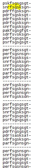
Should multiple amino acids have the same or close to the same frequency, the graph can get cluttered and difficult to interpret. Adjusting the Y axis can help clarify amino acid identity. At each position percentages may not add up to 100 depending on the number of gaps. Consider the sequence “RFSGS” at positions 69-73 which is in a region containing gaps for some of the clones:
u <- 80 u.s <- 110 u.prime <- 90 S <- u.s - u #selection differential R <- u.prime - u # response to selection h2 <- R/S #realized heritability h2 ## [1] 0.3333333
Problem 2
1 2 3 4 5 6 7 8
u <- 140 u.s <- 165 h2 <- 0.4 S <- u.s - u #selection differential R <- h2*S u.prime <- u + R u.prime ## [1] 150
If females only have u.s=165 and we assume males u=140 then the average u.s = (165+140)/2 = 152.5
1 2 3 4 5 6 7 8
u <- 140 u.s <- 152.5 h2 <- 0.4 S <- u.s - u #selection differential R <- h2*S u.prime <- u + R u.prime ## [1] 145
Problem 3
1 2 3 4 5 6 7 8
u <- 60 u.s <- 48 h2 <- 0.12 S <- u.s - u #selection differential R <- h2*S u.prime <- u + R u.prime ## [1] 58.56
Problem 4
1 2 3 4 5 6 7 8 9 10 11 12 13 14 15 16 17 18
u.s <- 35 u.prime <- 25 h2 <- 0.4
#S <- u.s - u #selection differential #R <- h2*S #u.prime <- u + R or R <- u.prime - u
#Rearrange to get:
#R <- h2*(u.s-u) #u.prime - u <- h2*(u.s-u) #solve for u:
u <-(u.prime-h2*u.s)/(1-h2) u ## [1] 18.33333
Problem 5
1 2 3 4 5 6 7 8 9 10 11 12 13
u <- 110 h2 <- 0.25 #S <- u.s - u #selection differential S <- 80 u.s <- S + u u.s ## [1] 190 R <- h2*S R ## [1] 20 u.prime <- u + R u.prime ## [1] 130
Problem 6
1 2 3 4 5 6 7 8 9 10 11 12 13 14 15 16 17 18 19
u <- 100 #S <- u.s - u #selection differential S <- 32 u.s <- S + u u.s ## [1] 132 #From Table IX p292 half sib covariance equals the additive genetic variance divided by 4 so
sigma2.a <- 12*4 sigma2.p <- 240 h2 <- sigma2.a/sigma2.p h2 ## [1] 0.2 R <- h2*S R ## [1] 6.4 u.prime <- u + R u.prime ## [1] 106.4
Narrow sense heritability $$\displaystyle h^2= \frac{\sigma^2_a}{\sigma^2_p}$$
If $$\displaystyle \sigma^2_d +\sigma^2_i = 0$$ then Broad sense heritability and narrow sense heritability are the same and so the maximum narrow sense is 0.7. Heritability can be zero, so the range is 0 - 0.7.
Problem 9
Narrow sense heritability $$\displaystyle h^2= \frac{\sigma^2_a}{\sigma^2_p}$$
cov(x,y)#5 covariance of x and y ## [1] -8.333333 cor(x,y)#6 correlation coefficient of x and y ## [1] -0.9708024 #7 the regression coefficient is the slope of the fit line, "y" in the summary output below. The correlation coefficient can also be extracted from the model.
model <- lm(x ~ y) model ## ## Call: ## lm(formula = x ~ y) ## ## Coefficients: ## (Intercept) y ## 17.110 -1.059
results <- data.frame(cbind(sample, response)) results ## sample response ## 1 a 6 ## 2 a 4 ## 3 a 2 ## 4 a 3 ## 5 b 5 ## 6 b 5 ## 7 b 3 ## 8 c 7 ## 9 c 6 ## 10 c 4 ## 11 c 5 ## 12 c 4
results.2 <- split(results, sample) results.2 ## $a ## sample response ## 1 a 6 ## 2 a 4 ## 3 a 2 ## 4 a 3 ## ## $b ## sample response ## 5 b 5 ## 6 b 5 ## 7 b 3 ## ## $c ## sample response ## 8 c 7 ## 9 c 6 ## 10 c 4 ## 11 c 5 ## 12 c 4 getWithinGroupSum <-function(x){#get the within group sum $\Sigma_jx_{ij}$ sum(as.numeric(unlist(x["response"])))}
## a b c ## 2.750000 3.333333 4.200000 getNsq <-function(x){ nrow(x)^2}
n.i.2 <- sapply(results.2, getNsq) n.i.2
## a b c ## 16 9 25 getWGDelta <-function(x){#within group difference from the group mean squared sum((as.numeric(unlist(x["response"]))- mean(as.numeric(unlist(x["response"]))))^2) }
WSS <-sum( sapply(results.2, getWGDelta)) WSS
## [1] 18.21667 grand.mean <- mean(as.numeric(results$response)) grand.mean #grand mean for all samples
$$\displaystyle \frac{d\bar{w}}{dp} = -2ps +2t -2tp = 0$$ Rearrange to get -2ps - 2pt =-2t or ps + pt = t or $$\displaystyle p = \frac{t}{s+t}$$ at equilbrium.
$$\displaystyle \frac{d^2\bar{w}}{dp^2} = -2s -2t < 0$$ so a maximum of $$\bar{w}$$
Box F
Problem a
Method
Formula
B=0.1
B=0.01
notes
Tandom
i
1.76
2.66
table p261
independent culling
ni’
3(0.88)=2.64
3(1.4)=4.2
B=0.45 ,i=0.88;B=0.2 ,i=1.4
index selection
i$$\sqrt{n}$$
3.05
4.6
Problem b
$$\displaystyle I = a_1h^2_1x_1 + a_2h^2_2x_2 = (81.57)(0.47)x_1 + (20.1)(0.47)x_2$$
N <- 1/((1/5)*(1/500+1/1500+1/10+1/50+1/1000)) N ## [1] 40.43127
Problem 3
1 2 3 4 5 6
p <-c(0.55,0.2,0.09,0.06,0.04,0.03,0.02,0.01)
#The effective number if alleles is 1/homozygosity; homozygosity = SUM[p2]
1/sum(p^2) ## [1] 2.799552
If each allele had the same frequency (0.125) and there are 8 alleles then the effective number of alleles is 8, as that is the definition of effective number.
$$\hat{p} = \frac{w_{12}-w_{22}}{2w_{12}-w_{11}-w_{22}}$$
With $w_{11}=0.98$ and $w_{12}=1$ and $\hat{p}=0.8$
$$0.8=\frac{1-w_{22}}{2(1)-0.98-w_{22}}$$
$$w_{22}=0.92$$
data <- data.frame( Group1, Group2, Group3, Group4, Group5)
#let's reshape the data so we can get a view of what we are analyzing data2 <- reshape(data, varying=list(names(data)), v.names="p", direction="long", timevar="Group")
#As the populations drift towards the extremes (p=0 or p=1) heterozygosity decreases. #calculate the total heterozygosity in the group #HT= 2*p.bar*(1-p.bar)
The R function dist() will calculate distance matrices using a variety of methods, none of which are the genetic distance we are interested in, exemplified by the equation:
$$d^2 = 1 - \sqrt{p_1p_2} - \sqrt{q_1q_2}$$
Therefore we need to define our own function “GeneticDistance”. I also represent the alleles as p.1 and p.2 only, to simplify the function.
Where $$\gamma$$ is Euler’s constant. To obtain Euler’s constant we will use the negative derivative of the gamma function evaluated at 1: -digamma(1), which equals ~0.5772157
1 2 3
s <- 0.01 2*(N.e/N.a)*log(2*N.a/(2*N.e*s))+1-(-digamma(1)) ## [1] 8.148086
i.e 8.148 generations.
Box F
Problem a
For the stepping stone model use $$\displaystyle\hat{F} \approx \frac{1}{4N\sqrt{2m\mu}+1}$$
For the island model use $$\displaystyle\hat{F} \approx \frac{1}{4N(m+\mu)+1}$$
Comparing neighborhood sizes in b (uniform population distribution in one dimension) and c (uniform population distribution in two dimensions) above:
1
2
3
4
5
6
7
8
9
10
11
12
13
14
15
16
17
u <- 1e-6 m <- 0.01 N <- 50 delta <- N sigma <-sqrt(m)
N.b <- 2*sqrt(pi)*delta*sigma N.b ## [1] 17.72454
delta <- 325 sigma <- 0.07
N.c <- 4*pi*sigma^2*delta N.c ## [1] 20.01195 #So the neighborhood size is effective the same for N= 50 (one dimension) and N=325 (two dimensions)
Box G
Problem a
$$\displaystyle p' = \frac{p(pw_{11} + qw_{12})}{\bar{w}}$$
Subtract p from both sides:
$$\displaystyle p'-p = \frac{p(pw_{11} + qw_{12})}{\bar{w}}-p$$
Multiply p by$$\frac{\bar{w}}{\bar{w}}$$ and rearrange to get:
$$\displaystyle \Delta p = \frac{1}{\bar{w}}[p(pw_{11} + qw_{12}) - p\bar{w} ]$$
Given that: $$\bar{w} = p^2w_{11} + 2pqw_{12} + q^2w_{22}$$
$$\displaystyle \Delta p = \frac{1}{\bar{w}}[p(pw_{11} + qw_{12}) - p(p^2w_{11} + 2pqw_{12} + q^2w_{22}) ]$$
$$\displaystyle \Delta p = \frac{1}{\bar{w}}[p^2w_{11} + pqw_{12} - pp^2w_{11} - 2p^2qw_{12} - pq^2w_{22} ]$$
$$\displaystyle \Delta p = \frac{1}{\bar{w}}[p^2w_{11} - pp^2w_{11} + pqw_{12} - 2ppqw_{12} - pq^2w_{22} ]$$
$$\displaystyle \Delta p = \frac{1}{\bar{w}}[w_{11}(p^2 - pp^2) + w_{12}(pq -2ppq) - pq^2w_{22} ]$$
$$\displaystyle \Delta p = \frac{1}{\bar{w}}[w_{11}p^2(1 - p) + w_{12}pq(1 -2p) - pq^2w_{22} ]$$
Given that $$1-2p=(1-p)-p=q-p$$:
$$\displaystyle \Delta p = \frac{1}{\bar{w}}[w_{11}p^2q + w_{12}pq(q -p) - pq^2w_{22} ]$$ then factor out pq to get:
$$\displaystyle \Delta p = \frac{pq}{\bar{w}}[w_{11}p + w_{12}(q -p) - qw_{22} ]$$
$$\displaystyle \Delta p = \frac{pq}{\bar{w}}[w_{11}p + w_{12}q -w_{12}p - qw_{22} ]$$
$$\displaystyle \Delta p = \frac{pq}{\bar{w}}[ p(w_{11} - w_{12}) +q(w_{12} - w_{22}) ]$$
Problem b
Part 1
$$\displaystyle w_{11}=w_{12}=1 \;\;\; w_{22}=1-s$$
$$\displaystyle\frac{dp}{dt} = pq^2s$$ or rearrange to $$\displaystyle\frac{dp}{pq^2}=s\; dt$$
So from $$t_0$$ to $$t_1$$:
$$\displaystyle\int_{p_0}^{p_t} \frac{1}{pq^2}dp = \int_{t_0}^{t_1} s\; dt$$
First the left hand integral. Given that:
$$\displaystyle\int \frac{1}{x(1-x)^2}\;dx = \frac{1}{1-x}-ln(\frac{1-x}{x})$$
Then $$\displaystyle\int_{p_0}^{p_t} \frac{1}{pq^2}dp =[\frac{1}{1-p_t}-ln(\frac{1-p_t}{p_t})]-[\frac{1}{1-p_0}-ln(\frac{1-p_0}{p_0})]$$
$$\displaystyle =\frac{1}{1-p_t} - ln(\frac{1-p_t}{p_t})- \frac{1}{1-p_0} + ln(\frac{1-p_0}{p_0}) = \frac{1}{q_t} - ln(\frac{q_t}{p_t}) - \frac{1}{q_0} + ln(\frac{q_0}{p_0})$$
Because $$ln(\frac{a}{b}) = ln(a) - ln (b)$$ and $$ln(ab) = ln(a)+ln(b)$$ simplify to:
$$\displaystyle = ln(\frac{p_tq_0}{p_0q_t}) + \frac{1}{q_t} - \frac{1}{q_0}$$
For the right hand integral:
$$\displaystyle \int_{t_0}^{t_1} s\; dt = s(t - 0) = st$$
Setting the two solutions equal gives:
$$\displaystyle st = ln(\frac{p_tq_0}{p_0q_t}) + \frac{1}{q_t} - \frac{1}{q_0}$$
Part 2
$$\displaystyle \frac{dp}{dt} = \frac{pqs}{2}$$ rearrange to get:
$$\displaystyle 2\frac{1}{pq};dp = s;dt$$
Right hand side as above. For the left side:
$$\displaystyle 2\int^{p_t}_{p_0}\frac{1}{p(1-p)} dp$$
Given that $$\displaystyle \int \frac{1}{x(1-x)}\;dx = -ln\frac{(1-x)}{x}$$
$$\displaystyle 2\int^{p_t}_{p_0}\frac{1}{p(1-p)}\;dp = 2[[-ln\frac{1-p_t}{p_t}]-[-ln\frac{1-p_0}{p_0}]]$$
$$\displaystyle = 2[ ln\frac{p_t}{1-p_t} + ln\frac{1-p_0}{p_0}]$$
$$\displaystyle = 2[ ln\frac{p_t}{q_t} + ln\frac{q_0}{p_0}]$$
$$\displaystyle = 2 ln\frac{p_tq_0}{q_tp_0}$$
Part 3
$$\displaystyle \frac{dp}{dt} = p^2qs$$ rearrange to get:
$$\displaystyle \frac{1}{p^2q}\;dp = s\;dt$$
Right hand side as above. We are also given that $$\displaystyle \int \frac{1}{x^2(1-x)}\;dx=-\frac{1}{x}-ln\frac{1-x}{x}$$ so:
$$\displaystyle \int^{p_t}_{p_0}\frac{1}{p^2(1-p)}\;dp = -\frac{1}{p_t} - ln\frac{1-p_t}{p_t}-[-\frac{1}{p_0} - ln\frac{1-p_0}{p_0}]$$
$$\displaystyle = -\frac{1}{p_t} - ln\frac{q_t}{p_t} + \frac{1}{p_0} + ln\frac{q_0}{p_0}$$
$$\displaystyle = -\frac{1}{p_t} + \frac{1}{p_0} + ln\frac{p_t}{q_t} + ln\frac{q_0}{p_0}$$
$$\displaystyle = -\frac{1}{p_t} + \frac{1}{p_0} + ln\frac{p_tq_0}{q_tp_0}$$
t <-(log((p.t*q.0)/(p.0*q.t))+1/q.t -1/q.0)/s t ## [1] 10818.01
#Part 2
t <-(2*log((p.t*q.0)/(p.0*q.t)))/s t ## [1] 1838.048
#Part 3
t <-(log((p.t*q.0)/(p.0*q.t))-1/p.t +1/p.0)/s t ## [1] 10818.01
#Part 4
t <-(log((p.t*q.0)/(p.0*q.t)))/s t ## [1] 919.024
Box H
Problem a
Given: $$P_t= P_{t-1}(1-\mu)+(1-P_{t-1})\nu$$
We want the expression for: $P_t - \frac{\nu}{\mu+\nu}$ so subtract $\frac{\nu}{\mu+\nu}$ from both sides of the given equation.
$$p_t - \frac{\nu}{\mu+\nu} = p_{t-1}(1-\mu)+(1-p_{t-1})\nu - \frac{\nu}{\mu+\nu}$$
$$p_t - \frac{\nu}{\mu+\nu} = p_{t-1}- \mu p_{t-1} + \nu - \nu p_{t-1} - \frac{\nu}{\mu + \nu}$$
$$p_t - \frac{\nu}{\mu+\nu} = p_{t-1}(1 - \mu - \nu ) + \nu - \frac{\nu}{\mu + \nu}$$
$$p_t - \frac{\nu}{\mu+\nu} = p_{t-1}(1 - \mu - \nu ) + \frac{\nu(\mu + \nu)}{\mu + \nu} - \frac{\nu}{\mu + \nu}$$
$$p_t - \frac{\nu}{\mu+\nu} = p_{t-1}(1 - \mu - \nu ) + \frac{\nu\mu + \nu^2 - \nu}{\mu + \nu}$$
$$p_t - \frac{\nu}{\mu+\nu} = p_{t-1}(1 - \mu - \nu ) - \frac{\nu(1 - \mu - \nu)}{\mu + \nu}$$
$$p_t - \frac{\nu}{\mu+\nu} = [p_{t-1} - \frac{\nu}{\mu + \nu}](1 - \mu - \nu)$$
So $a=\frac{\nu}{\nu+\mu}$ and $b=(1-\mu-\nu)$
Given: $p_t - a = (p_0-a)b^t$ substitute to get:
$$p_t - \frac{\nu}{\mu+\nu} = [p_0 - \frac{\nu}{\mu + \nu}](1 - \mu - \nu)^t$$
### Problem b ###
$$p_t = p_{t-1}(1-m)+\bar{p}m$$
We are interested in $p_t - \bar{p}$ so subtract $\bar{p}$ from both sides.
$$p_t - \bar{p} = p_{t-1}(1-m)+\bar{p}m - \bar{p}$$
$$p_t - \bar{p} = p_{t-1}(1-m)+\bar{p}(m - 1)$$
$$p_t - \bar{p} = p_{t-1}(1-m)-\bar{p}(1 - m)$$
$$p_t - \bar{p} = (p_{t-1} - \bar{p})(1-m)$$
So $a=\bar{p}$ and $b=(1-m)$
$$p_t - \bar{p} = (p_{0} - \bar{p})(1-m)^t$$
Divide both sides by $\bar{p}$:
$$\frac{p_t}{\bar{p}} - 1 = (\frac{p_0}{\bar{p}} -1)(1-m)^t$$
$$\frac{p_t}{\bar{p}} = (\frac{p_0}{\bar{p}} -1)(1-m)^t + 1$$
If $\frac{p_0}{\bar{p}}=2$, m=0.01, and t=69:
$$\frac{p_t}{\bar{p}} = (2 -1)(1-0.01)^{69} + 1= 1.499$$
Problem c
Box I
A fitness is $w_{11}$
a fitness is $w_{22}$
$$w=\frac{w_{11}}{w_{22}}$$
Given: $p_t = \frac{p_{t-1}w_{11}}{\bar{w}}$ and $q_t = \frac{q_{t-1}w_{22}}{\bar{w}}$
$$\frac{p_t}{q_t} = \frac{\frac{p_{t-1}w_{11}}{\bar{w}}}{\frac{q_{t-1}w_{22}}{\bar{w}}} = \frac{p_{t-1}w_{11}}{\bar{w}}\frac{\bar{w}}{q_{t-1}w_{22}} = \frac{p_{t-1}}{q_{t-1}}\frac{w_{11}}{w_{22}} = \frac{p_{t-1}}{q_{t-1}}w$$
Given: $\displaystyle \frac{p_t}{q_t}=\frac{p_0}{q_0}w^t$ take the natural ln of bothh sides:
Given: $\displaystyle ln(\frac{p_t}{q_t})=ln(\frac{p_0}{q_0}) + t ln(w)$
For a line y=mx + b where m=slope and b = y intercept
For the plot of $\displaystyle ln(\frac{p_t}{q_t})$ vs t:
Slope = m = $\displaystyle \frac{y_1-y_0}{x_1-x_0} = ln(w)$
Y intercept = b = $\displaystyle y_0 -mx_0= ln(\frac{p_0}{q_0})$
Two timepoints are given, call them $t_1$ and $t_2$
Use them to calculate the slope and y intercept. Then use the above equations to calculate $p_0$
#at t=5 #p.1/(1-p.1) = (p.0/q.0)*w^t.1 # set pq <- p.0/q.0 so pq <- p.1/((1-p.1)*w^t.1) pq ## [1] 0.6393112
#so pq or p.0/q.0 or p.0/(1-p.0) = 0.6393 solve for p.0 p.0 <- 0.6393/1.6393 p.0 ## [1] 0.3899835
q.0 <- 1-p.0 q.0 ## [1] 0.6100165
#calculate y intercept
b <-log(p.0/q.0) b ## [1] -0.4473815
#Since the A and a strains were originally equal in fitness, i.e. w=1 #now that w=1.149 that is an increase of 0.149 per 120 generations #per generation: (w-1)/120#fitness units per generation ## [1] 0.001238077
(w-1)/120*100#percent per generation ## [1] 0.1238077
Box J
For L(mutation):
L(mutation) = $$\displaystyle \mu$$ = 2e-6
$$\displaystyle \hat{q}=\sqrt{\frac{\mu}{s}}$$
1 2 3 4 5 6 7 8
u <- 2e-6 s <- 0.0052 q.hat <-sqrt(u/s) q.hat ## [1] 0.01961161 L.mut <- u L.mut ## [1] 2e-06
model <-lm(legit ~ distance ) summary(model) ## ## Call: ## lm(formula = legit ~ distance) ## ## Residuals: ## ALL 2 residuals are 0: no residual degrees of freedom! ## ## Coefficients: ## Estimate Std. Error t value Pr(>|t|) ## (Intercept) 5.42e-01 NA NA NA ## distance -7.05e-05 NA NA NA ## ## Residual standard error: NaN on 0 degrees of freedom ## Multiple R-squared: 1, Adjusted R-squared: NaN ## F-statistic: NaN on 1 and 0 DF, p-value: NA
#using y=mx + b where m:slope, b:y-intercept b <- model[[1]][1] b[[1]] ## [1] 0.542
m <- model[[1]][2] m[[1]] ## [1] -7.05e-05
a <- 1/abs(m)#the distance along a cline corresponding to an allele frequency change of 1 legit, measured in kilometers. a[[1]] ## [1] 14184.4 #use the reported variance of 10 km^2 v <- 10 g <- 4*v/a^3 g[[1]]# per kilometer ## [1] 1.40161e-11 #percent change across the distance 2000*g[[1]] ## [1] 2.803221e-08
phenotypes <-c("pp","pq","qq") observed <-c(9999,1)#9999 is pp + pq count total <-sum(observed)
Freq.q <-sqrt(1/total) Freq.q
1
## [1] 0.01
1 2
Freq.p <- 1-Freq.q Freq.p
1
## [1] 0.99
1 2
heterozygotes <- 2*Freq.p*Freq.q heterozygotes
1
## [1] 0.0198
Therefore about 2% of the Caucasian population is a carrier (~1/50)
## Problem 8 ##
1
2
3
4
5
6
7
8
9
10
11
12
A1 <- 0.1 A2 <- 0.2 A3 <- 0.3 A4 <- 0.4
alleles <-c( A1, A2, A3, A4 )
#here is a hack to get at the frequencies more effortlessly (maybe) #take the outer product of the vector 'alleles'. This will multiply all #combinations of alleles e.g. all p*q combinations. initial <- alleles %o% alleles initial
#This is correct for homozygotes e.g. p^2 (on the diagonal), but heterozygotes are 2pq. #All elements of the matrix except the diagonal need to be multiplied #by 2, the diagonal by 1 # multiplier <- matrix(2, nrow=4, ncol=4) diag(multiplier)<-1 multiplier
## aGpdh amy NS counts ## 1 F F non-NS 726 ## 2 F F NS 90 ## 3 F S non-NS 111 ## 4 F S NS 1 ## 5 S F non-NS 172 ## 6 S F NS 32 ## 7 S S non-NS 26 ## 8 S S NS 0
1 2 3 4 5 6 7 8 9 10 11 12
#calculate the total number of observations total <-sum(results$counts) total ## [1] 1158
#part b: calculate the aGpdh (F)ast and (S)low frequencies
#s probability of survival from age class i to i+1 s <-c(0.5,0.5,0.5,0.5,0)
# b is the average number of offspring born to an individual in age class i
b <-c(0,1,1.5,1,0)
#using the characteristic equation, create a vector ce where each element holds an element of the equation. As there are 5 elements create a 5 element vector
Using the table I extract coefficients fromt the “Offspring Frequency” Aa column and apply to the “Frequency of Mating” column to obtain the frequency of heterozygotes in the next generation, Q’:
# note that we are no longer interested in aGpdh. # use aGpdh as a "replicates" indicator and reprocess the table to combine replicate #counts prior to calculating frequencies
#D <- P11 - p1q1, -.011794 # Let's use amy "F" and NS "non-NS" as P11. and calculate D from there # First, pull ot the relevent row then calculate the ratio
chisq.test( observed, p = expected, rescale.p=TRUE, correct=FALSE)
1 2 3 4 5
## ## Chi-squared test for given probabilities ## ## data: observed ## X-squared = 16.165, df = 3, p-value = 0.001049
Problem E
This is the same as E only now we use aGpdh instead of amy
1 2 3 4 5 6 7 8
# note that we are no longer interested in amy. # use amy as a "replicates" indicator and reprocess the table to combine replicate #counts prior to calculating frequencies
chisq.test( observed, p = expected, rescale.p=TRUE, correct=FALSE)
1 2 3 4 5
## ## Chi-squared test for given probabilities ## ## data: observed ## X-squared = 3.2748, df = 3, p-value = 0.3512
Note that the degrees of freedom of 3 used by R is inappropriate. For 1 degree of freedon (4 - 1 (sample size) -1 (estimating p1) -1 (estimating p2) = 1 ) you must read a p ~0.07 off a chi square table. Do not reject the null hypothesis ( independence or linkage equilibrium) and so conclude linkage equilibrium.
Let’s try a brute force approach. Populate a vector of length 1000 with 250 AA, 500 Aa and 250 aa. Sample with replacement 1000 times 6 geneotype. Calculate the fraction with aa present 2 or fewer times.
1 2 3 4 5 6 7 8 9 10 11 12 13 14 15 16 17
population <-c(rep("AA",250),rep("Aa",500),rep("aa",250)) counts <- vector( mode='character',length=1000)
for( i in1:1000){
my.sample <- sample(population,6, replace=TRUE) counts[i]<-length( which(my.sample=="aa"))#each element of the vector "counts" holds the number of aa genotypes in the sample }
table(counts)#provides the counts of each genotype ## counts ## 0 1 2 3 4 5 ## 185 345 298 127 42 3 total.counts <- table(counts)[[1]]+ table(counts)[[2]]+ table(counts)[[3]] total.counts #of aa 2 or fewer times. Divide by 1000 to get percentage ## [1] 828
## Problem 4
Jack, queen, king are the face cards so Jack is likely 1/3 of the time a face card is drawn.
There are 4 Jacks so Jack of Hearts is 1 of 4.
The probability that a randomly drawn face card (of which there are 12) is the jack of hearts is 1 of 12.
Figure out potentially relevant probabilities then answer the question.
P{FaceCard}: probability of a Face card = 12/52 = 3/13
P{Jack}: probability of a Jack = 4/52 = 1/13.
P{Hearts}: probability of a hearts = 13/52 = 1/4.
P{Jack | FaceCard}: probability of a Jack given it’s a face card = 4/12 = 1/3.
P{Jack | Hearts}: probability of a Jack given it’s a heart = 1/13.
P{Heart | Jack}: probability of a heart given a Jack = 1/4
P{FaceCard | Jack}: probability of a face card given it’s a Jack = 1
What is the probability that a randomly drawn face card is the jack of hearts?
P{JackHearts | FaceCard} = P{ Heart | Jack } X P{Jack | FaceCard} = 1/4 x 1/3 = 1/12
What is the probability of a Jack given a face card?
There are 12 Face cards and 4 are Jacks so 4/12 or 1/3
Rewrite the Bayesian rule as: P{Jack|FaceCard} = P{FaceCard|Jack}*P{Jack}/P{FaceCard}
P{Jack|FaceCard} = (1*1/13)/3/13 = 1/3
## Problem 6
1 2 3 4 5 6 7 8 9 10 11 12 13 14 15 16 17
observed <-c(60,40) #expected <- c(50, 50) #expected with independent assortment expected <-c(0.5,0.5)#R expects frequencies that add to one
chisq.test( observed, p = expected, correct=FALSE) ## ## Chi-squared test for given probabilities ## ## data: observed ## X-squared = 4, df = 1, p-value = 0.0455 chisq.test( observed, correct=FALSE)#since equal frequencies is the default, p does not need to be specified' ## ## Chi-squared test for given probabilities ## ## data: observed ## X-squared = 4, df = 1, p-value = 0.0455
r = 40/100 = 0.4
standard error = sqrt(( 0.4*( 1-0.4 ))/100 = 0.049
template <-"tactgtgaaagatttccgact" #the comp and many other seqinr functions require a vector of characters #convert a string to vector of characters using s2c (sequence 2 character). c2s converts a vector back to a string.
template.complement <- comp(s2c(template)) template.complement ## [1] "a" "t" "g" "a" "c" "a" "c" "t" "t" "t" "c" "t" "a" "a" "a" "g" "g" ## [18] "c" "t" "g" "a" template.complement <- c2s(comp(s2c(template))) template.complement ## [1] "atgacactttctaaaggctga" # FRAME is 0,1, or 2
c2s(translate( s2c(template.complement), frame=0)) ## [1] "MTLSKG*" c2s(translate( s2c(template.complement), frame=1)) ## [1] "*HFLKA" #substitute an A for the first G in template
template.subs.g <- sub("g","a", template) template.subs.g ## [1] "tactatgaaagatttccgact" template.subs.g.comp <- c2s(comp(s2c(template.subs.g))) template.subs.g.comp ## [1] "atgatactttctaaaggctga" c2s(translate( s2c(template.subs.g.comp), frame=0)) ## [1] "MILSKG*" template.subs.a <- sub("c","ca", template) template.subs.a ## [1] "tacatgtgaaagatttccgact" template.subs.a.comp <- c2s(comp(s2c(template.subs.a))) template.subs.a.comp ## [1] "atgtacactttctaaaggctga" c2s(translate( s2c(template.subs.a.comp), frame=0)) ## [1] "MYTF*RL" #When the frame is unknown, but a particular amino acid motif is desired, the "getFrame" method can be used to identify the proper frame.
getFrame <-function( pattern, seq){
#seq must be character vector of lower case dna (not a seqFastdna object) #pattern is the amino acid sequence in capital letters #return 0,1,2 for frames 1,2,3 #return 3 if present in more than one frame #return 4 if not present
fr <-c(NA,NA,NA)
for( i in1:3){ fr[i]<- words.pos(pattern, c2s(translate( seq, frame=i-1, sens="F")))[1] }
if(length( which(!is.na(fr), arr.ind=TRUE))==1){ result <- which(!is.na(fr), arr.ind=TRUE)-1#subtract one because seqinar uses 0,1,2 as frames }else{ if(length( which(!is.na(fr), arr.ind=TRUE))>1){ result <- 3 }else{ result <-4}} return(result) }
#The original template provides a translation with the motif "LSK" #Translate in the frame containing this motif
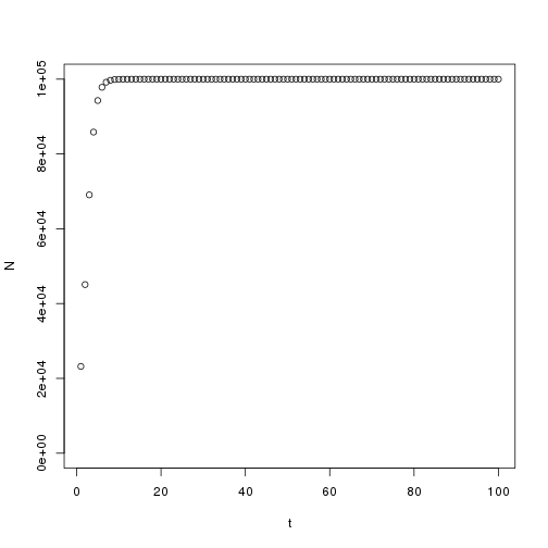
K <- 100000 N.0 <- 10000 t <- 1:100 C <-(K-N.0)/N.0 r <- 1 N <- vector("numeric",100)
N[t]<- K/(1+ C*exp(-r*t))
plot(t, N, ylim=c(0,100000))
1 2 3 4
#Let's change the rate to 0.1 r <- 0.1 N[t]<- K/(1+ C*exp(-r*t)) plot(t, N, ylim=c(0,100000))
1 2 3 4 5
#It takes longer to reach the carrying capacity #Let's change the rate to -0.1 r <--0.1 N[t]<- K/(1+ C*exp(-r*t)) plot(t, N, ylim=c(0,100000))
1 2 3 4 5 6 7 8 9 10
#The population crashes to 0
#What if N.0 > K (rate is positive)
K <- 10000 N.0 <- 20000 r <- 1 C <-(K-N.0)/N.0 N[t]<- K/(1+ C*exp(-r*t)) plot(t, N, ylim=c(0,20000))
1
#Population drops to the carrying capacity
## Problem 14
1 2 3 4 5 6 7 8 9
observed <-c(88,37) expected <-c(0.75,0.25) chisq.test( observed, p = expected, correct=FALSE) ## ## Chi-squared test for given probabilities ## ## data: observed ## X-squared = 1.4107, df = 1, p-value = 0.2349 #Accept the hypothesis of Mendelian segregation
## Problem 15
1
2
3
4
5
6
7
8
observed <-c(269,98,86,88,30,34,27,7) expected <-c(27/64,9/64,9/64,9/64,3/64,3/64,3/64,1/64)#probabilities must sum to 1 chisq.test( observed, p = expected, correct=FALSE) ## ## Chi-squared test for given probabilities ## ## data: observed ## X-squared = 2.673, df = 7, p-value = 0.9135