QPix2 Part 2

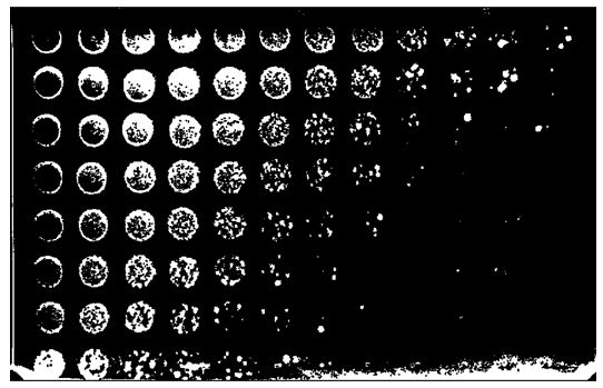
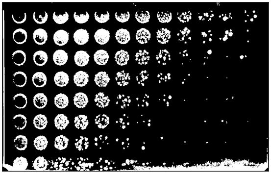
The QPix software identifies a single region per plate (two regions total) and randomly picks a user defined number of colonies from each region. Ideally one would want to define 96 regions per plate so that the number of colonies per region can be specified - not allowed. However each colony’s location (X|Y deck coordinate) is recorded in an XML log file.

With a bit of hacking, the well location can be assigned to each colony. In this post I will process the XML log file to extract X|Y coordinates for each picked colony, associate those coordinates with wells, associate clone IDs with wells and ultimately associate the clone ID with a picked colony.

See this post for details concerning the input files and custom methods.

1
2
3
4
5
6
7
8
9
10
11
12
13
14
15
16
17
18
19
20
21
22
23
24
25
rm(list=ls(all=TRUE))
library(XML)

setwd('~./qpix2')
#this is the files that indicates the clone IDs of the VH, VL fragments that
#have been cloned - the ID of the transformation mix
assoc.file <- "amplicon-plate-map.txt"
assoc <- read.table( paste(getwd(),"input", assoc.file, sep="/"), skip=0, header=TRUE)

> assoc
id dest.plate dest.well
1 PL101-VH amplicons A01
2 PL102-VH amplicons B01
3 PL103-VH amplicons C01
4 PL18-VH amplicons D01
5 PL28-VH amplicons E01
6 PL38-VH amplicons F01


##extract the runid as six integers
qpix.filename <- "QSoft Log 2014-02-11 105201.XML"
runid <- substring( qpix.filename, 22, 27)
> runid
[1] "105201"

Supply plate names of the plates in which the picked colonies were deposited. This is not needed if the plate names are typed directly into the software. For this example I will assume they are not. Enter as many destination plates as exist, the script will adjust

1
2
3
4

dest.plate <- list()
dest.plate[[1]] <- "PL140211c"
dest.plate[[2]] <- "PL140211d"

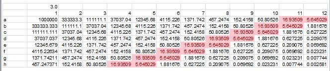
Use region 2 well H01 as the “origin”. Enter calibration block values for well G01. From G01 calculate H01 using hard coded offsets.

1
2
3
4
5
6
7
8
9
10
11
12
13
14
15
16
17

g01.x <- 114278
g01.y <- 241732
xstart <- g01.x + 2580
ystart <- g01.y - 8781
> xstart
[1] 116858
> ystart
[1] 232951

d <- xmlTreeParse( paste(getwd(), "/qpix-logs/", qpix.filename, sep="") )
top <- xmlRoot(d)
##top[[11]] has the "contents"; should be as many deposits as destination plates
>names(top[[11]])
routine imaging colonydata deposit deposit
"routine" "imaging" "colonydata" "deposit" "deposit"
>

Retrieve XML log files off the Qpix post run. Colony data is in //contents/colonydata. The XML can be easily visulaized by opening with a browser. Colonydata contains X|Y location as well as region. Read it in and create a dataframe.

1
2
3
4
5
6
7
8
9
10
11
12
13
14
15
colony.data <- getNodeSet(top, "//contents/colonydata")
d2 <- data.frame(t(sapply( xmlApply(colony.data[[1]], xmlAttrs),c)), stringsAsFactors=FALSE)
# region-image-colonyid uniquely identifies a colony
# not sure why image is needed
d2 <- d2[,c("colonyid","image","posx","posy","region")]

> head(d2)
colonyid image posx posy region
1 0 5 159286 385817 1
2 1 5 159569 403677 1
3 2 5 160654 385588 1
4 3 5 160761 388800 1
5 4 5 160854 371823 1
6 5 5 161284 390663 1
>

Calculate centers of each column along X axis.
Offset between regions 1 and 2 is 108174um.
The custom method getDeckWell defined here
Add the source well to the dataframe.

1
2
3
4
5
6
7
8
9
10
11
12
13
14
15
16
17
18
19
20
21
22
23
24
25
26
27
28
29
30
31
32
33
34
35
36
37

x.cent <- seq( xstart, by=9100, length.out=12)
yr1.cent <- seq( ystart+108174, by=9100, length.out=8)
yr2.cent <- seq( ystart, by=9100, length.out=8)

src.well <- rep( NA, nrow(d2))

for( i in 1:nrow(d2)){
src.well[i] <- getDeckWell( as.numeric(d2[ i, "posx"][[1]]), as.numeric(d2[ i, "posy"][[1]]), as.numeric(d2[ i, "region"][[1]]))
}
d2 <- cbind( d2, src.well)

> head(d2)
colonyid image posx posy region src.well
1 0 5 159286 385817 1 C06
2 1 5 159569 403677 1 A06
3 2 5 160654 385588 1 C06
4 3 5 160761 388800 1 C06
5 4 5 160854 371823 1 E06
6 5 5 161284 390663 1 C06
>

d2.wid <- merge( d2, assoc, by.x="src.well", by.y="dest.well")

> d2.wid
id colonyid src.well
1 PL101-VH 153 A01
2 PL101-VH 162 A01
3 PL101-VH 157 A01
4 PL101-VH 166 A01
5 PL101-VH 160 A01
6 PL44-VH 208 A02
7 PL44-VH 181 A02
8 PL44-VH 206 A02
9 PL44-VH 187 A02
10 PL44-VH 171 A02

Now we have associated an id based on well location to each colony.
src.well here is the well the clone came from in the transformation plate.
All we need here is colonyid assigned by Qpix and my clone id
src.well is the transformation well, keep that so you can
retrieve colonies that weren’t recovered by the Qpix.

1
2
3
4
5
6
7
8
9
10
11
12
13
14
15
16
17
18
19
20
21
22
23
24
25
26
27
28
29
30
31
32
33
34
35
36
37
38
39
40
41
42
43
44
45
46
47
48
49
50
51
52
53
54

d2.wid <- d2.wid[,c("id","colonyid","src.well")]
deposit <-getNodeSet(top, "//contents/deposit")

deposit.list <- list()
for( i in 1: length(deposit)){
deposit.list[[i]] <- data.frame(t(sapply( xmlApply(deposit[[i]], xmlAttrs),c)), stringsAsFactors=FALSE)
}

#may not need to do this if destinations entered in software
for(i in 1:length(deposit.list)){
deposit.list[[i]]$destination <- dest.plate[[i]]
}

d3 <- do.call("rbind", deposit.list)


d3$location <- sapply( d3$location, insert0inWell)

> head(d3)
destination location colonyid source region
1 PL140211c A01 0 UIDUO0211-3912159-X 1
2 PL140211c B01 1 UIDUO0211-3912159-X 1
3 PL140211c C01 2 UIDUO0211-3912159-X 1
4 PL140211c D01 3 UIDUO0211-3912159-X 1
5 PL140211c E01 4 UIDUO0211-3912159-X 1
6 PL140211c F01 5 UIDUO0211-3912159-X 1

d4 <- merge(d3, d2.wid, by.x="colonyid", by.y="colonyid")
d4 <- d4[,c("destination","location","id","src.well")] #src.well is the transformation well
d4 <- d4[ order( d4$destination, d4$location),]
names(d4)[1:2] <- c("plate","well")
> head(d4)
plate well id src.well
1 PL140211c A01 PL78-VL C06
137 PL140211c A02 PL44-VL A06
51 PL140211c A03 PL86-VL C07
86 PL140211c A04 PL86-VL C07
95 PL140211c A05 PL95-VL D08
104 PL140211c A06 PL94-VL C08

results <- as.data.frame(table(d4$src.well))
results <- results[ order( results$Freq),]

> results
Var1 Freq
1 A01 0
15 C02 0
22 C09 0
26 D04 0
31 D09 0
40 E09 0
41 E10 0

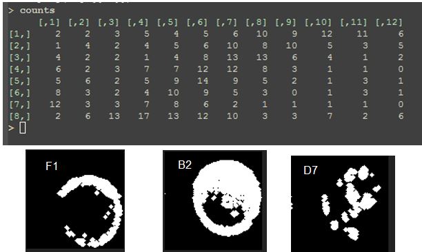
Results shows the count of colonies obtained per clone ID. Some are not present in the collection, as can be seen above where Freq==0. This provides a list of wells that can be plated manually if these are considered valuable colonies.

Pick out 4 candidates (if available) for each clone ID.

1
2
3
4
5
6
7
8
9
10
11
12
13
14
15
16
17
18
19
d5 <- do.call("rbind", lapply( split( d4, d4$bdn ), function(x) x[1:4,]) )
d5 <- d5[ !is.na(d5$bdn),]
d5 <- d5[ order( d5$plate, d5$well ),]

##evaluate
set1 <- read.table( paste(getwd(), "103410-picked-plates-map.txt", sep=""), skip=0, header=TRUE)
set2 <- read.table( paste(getwd(), "105201-picked-plates-map.txt", sep=""), skip=0, header=TRUE)

composite <- rbind(set1, set2)
out.file <-paste( working.dir, "composite.txt", sep="")
write.table( composite, file = out.file, append = FALSE, quote = FALSE, sep = "\t", eol = "\n", na = "NA", dec = ".", row.names = FALSE, col.names = TRUE, qmethod = c("escape", "double"))


results <- as.data.frame(table(composite$src.well))
results <- results[ order( results$Freq),]

plot(results)

set1 and set2 provide the plate maps for the picked plates.
results show the number of colonies picked for each candidate id. For those with 0-2 colonies, manually pick supplemental colonies if available.

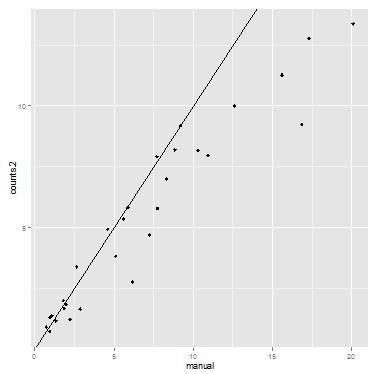
results can be plotted to get a sense for the distribution of colony counts for the various candidate clones.

Share

QPix2 setup

In this post I will provide some setup information for a later post that will discuss extracting clone IDs from a Qpix XML log file. This post consists of two sections, input files and custom methods.

Input files

Plate map file

The amplicon plate map provides the clone ID associated with the PCR product in each well of the 96 well pcr plate. This is the ID that ultimately you would like to associate with a colony.

1
2
3
4
5
6
7
8
9
10
11
assoc.file <- "amplicon-plate-map.txt"
assoc <- read.table( paste(getwd(),"input", assoc.file, sep="\\"), skip=0, header=TRUE)
> assoc
id dest.plate dest.well
1 PL101-VH amplicons A01
2 PL102-VH amplicons B01
3 PL103-VH amplicons C01
4 PL18-VH amplicons D01
5 PL28-VH amplicons E01
6 PL38-VH amplicons F01

QPix2 XML files

These are the log files retrieved from the Qpix post run.

[Example 1](QSoft Log 2014-02-11 103410.XML)
[Example 2](QSoft Log 2014-02-11 105201.XML)

Useful Methods

getDeckWell()

1
2
3
4
5
6
7
8
9
10
11
12
13
14
getDeckWell <- function( x, y, region){
#region is 1 or 2
cols <- c("01","02","03","04","05","06","07","08","09","10","11","12")
rows <- c("H","G","F","E","D","C","B","A")
##note that if a colony has equal but opposite sign offsets with two columns, this algorithm will fail!!
x.offset <- x.cent-x
y.offset <- switch( region,
"1" = yr1.cent-y,
"2" = yr2.cent-y)

paste(rows[ which(abs(y.offset)==min(abs(y.offset)))],
cols[ which(abs(x.offset)==min(abs(x.offset)))], sep="")

}

getWell96()

The function returns the opposite of what was supplied as a well ID i.e. provide well number get back the three character well ID. Provide three character well ID get back well number.

First create a table associating the three character well ID with well number.

1
2
3
4
5
6
7
8
9
10
> well.ids
name n
1 A01 1
2 B01 2
3 C01 3
4 D01 4
5 E01 5
6 F01 6
7 G01 7
8 H01 8

Once the table is defined, lookup either integer or three character well ID using the function argument.

1
2
3
4
5
6
7
8
9
10
11
12
getWell96 <- function( id ){
n <- 1:96
row <- rep(LETTERS[1:8],12)
col <- sort(rep(1:12, 8))
zero <- c(rep(0,72), rep("",24))
name <- I(paste(row,zero,col, sep="")) #I() is as.is to prevent factorization
well.ids <- data.frame(name, n)

if( id %in% name) {well.ids[well.ids$name==id,"n"]
}else{
well.ids[well.ids$n==id,"name"]}
}

insert0inWell()

Work only with three character well IDs e.g. A01, not A1. insert0inWell will insert a “0” in a 2 character well ID.

1
2
3
4
insert0inWell <- function( id){
if( nchar(id) == 2 ){ paste( substr(id, 1,1), "0", substr(id, 2,2), sep="")
}else{ id }
}
Share

QPix2 Introduction

In a previous post I showed how to use Omni plates to titer bacteria. Another useful application of OMNI plates is to plate out transformation mixes. In a high-throughput (96 well) cloning process it is easy to run In-Fusion reactions and transform bacteria in 96 well format. Vendors provide competent cells for chemical transformation in 96 well format. The bottleneck is plating and picking colonies. OMNI plates can be used to plate out 96 individual cloning reactions per OMNI plate.

The bottleneck then shifts to the next activity - picking colonies for sequencing. A Qpix2 colony picker can be used for picking. The Qpix deck will hold 2 OMNI plates using an Omni tray holder:

The software identifies a single region per plate (two regions total) and randomly picks a user defined number of colonies from each region. Ideally one would want to define 96 regions per plate so that the number of colonies per region can be specified - this is not allowed. However, each colonies location (X|Y deck coordinate) is recorded in an XML log file, and with a bit of hacking, the well location can be assigned to each colony.

The first step is to determine the how to interpret the coordinate system of the deck. I start by placing an agar filled OMNI plate on the deck of a BiomekNX liquid handling robot. Load the head with P20 tips and impale the surface of the agar.

The indentations on the surface of the agar are (mis)interpreted by the software as a colony and the X/Y cordinate will be reported. From this data one can determine the X|Y layout of the deck.

Now I can determine the coordinate boundaries for each of the 96 regions of interest:

More generally I can determine the coordinate layour of the entire deck. The coordinate system appears to be upside down, not surprising given that well A01 for each plate is bottom right corner. Apparently the engineers were standing at the back of the instrument during the design process. This has not been corrected in the newer version.

Now knowing the coordinates of the center of each well, I can assign an area to each well, and a well id to each colony that falls within that area.

I will assign an anchor coordinate and calculate everything as an offset to that. What if a PM or service call changes the deck slighly? I would like a way to calibrate. I find that I can use an ABI PCR plate holder as a calibration tool. Place the holder in the OMNI plate, scan, and the image can be used to assign an anchor coordinate. Because row H is too close to the edge of the image, “colonies” (actually the holes in the ABI plate) are not identified, so I use well G01 as my calibrator.

I can then calculate the offset between the ABI plate and the impaled OMNI plate. Should the coordinates of the ABI plate well G01 ever change, the change can be incorporated as an offset in the scripts.

Using this method I can assign source wells to the colonies I have picked and look at the pattern of deposit into the destination plate.

In this image the X|Y coordinates correspond to the OMNI plate e.g. OMNI plate well A01 is in the upper left corner, and the well ID is from the source plate. So the transformation mix from well D12 was deposited at position A01 on the OMNI plate. Looking at the pattern, I see no logic to it. Molecular Devices claims the picking order is optimized for speed.

Share

cheers

Here is an image from an advertisement from the early to mid oughts for the object database ObjectStore:

We (colleagues and I) speculated as to when we would be able to query images based on content. Who are these guys? What are they celebrating? What year is it? Where does the celebration take place? TinEye to the rescue:

Four international cocktail experts tasting some new drinks at the Wines, Spirits and Catering Trades Exhibition at Dorland Hall, London. October 30, 1933

Share

Change

Share

I am relevant

Share

Worst day at work - ever!

Share

Sequence evaluation

When processing sequences obtained from a vendor, it is useful to have an idea of how well the sequencing reactions worked, both in an absolute sense and relative to other recently obtained sequences in the same project. What follows is a primary sequence independent method of evaluating a collection (i.e. and order from an outside vendor) of sequences.

The first step is to align sequences by nucleotide index (ignoring the actual sequence). Start by reading the sequences into a list. I use the list s.b to hold forward (5’ to 3’) sequences, and the list s.f to hold the reverse (but in the 5’ to 3’ orientation, as sequenced) sequences:

1
2
3
4
5
6
7
8
9
10
11
12
13
14
15
16
17
18
19
20
21
rm(list=ls(all=TRUE))
library(seqinr)

working.dir <- "B:/<my-working-dir>/"


back.files <- list.files( paste(working.dir, "back/", sep="" ))
for.files <- list.files( paste(working.dir, "for/", sep="" ))

> back.files[1:20]
[1] "MBC20120428a-A1-PXMF1.seq" "MBC20120428a-A10-PXMF1.seq"
[3] "MBC20120428a-A11-PXMF1.seq" "MBC20120428a-A12-PXMF1.seq"
[5] "MBC20120428a-A2-PXMF1.seq" "MBC20120428a-A3-PXMF1.seq"
[7] "MBC20120428a-A4-PXMF1.seq" "MBC20120428a-A5-PXMF1.seq"
[9] "MBC20120428a-A6-PXMF1.seq" "MBC20120428a-A7-PXMF1.seq"
[11] "MBC20120428a-A8-PXMF1.seq" "MBC20120428a-A9-PXMF1.seq"
[13] "MBC20120428a-B1-PXMF1.seq" "MBC20120428a-B10-PXMF1.seq"
[15] "MBC20120428a-B11-PXMF1.seq" "MBC20120428a-B12-PXMF1.seq"
[17] "MBC20120428a-B2-PXMF1.seq" "MBC20120428a-B3-PXMF1.seq"
[19] "MBC20120428a-B4-PXMF1.seq" "MBC20120428a-B5-PXMF1.seq"
>

Next determine the number of files read and create a list of that length to hold the sequences. Then read them in and inspect a sequence:

1
2
3
4
5
6
7
8
9
10
11
12
13
14
15
16
17
18
19
20
21
22
23
24
25
26
27
28
s.b <- list()
length(s.b) <- length(back.files)
s.f <- list()
length(s.f) <- length(for.files)

for(i in 1:length(back.files)){
s.b[[i]] <- read.fasta(paste( working.dir, "back/", back.files[[i]], sep=""))
}

for(i in 1:length(for.files)){
s.f[[i]] <- read.fasta(paste( working.dir, "for/", for.files[[i]], sep=""))
}

> getSequence(s.b[[2]])[[1]][1:200]
[1] "n" "n" "n" "n" "n" "n" "n" "n" "n" "n" "n" "n" "n" "n" "c" "n" "n" "n"
[19] "g" "t" "c" "c" "a" "c" "t" "g" "c" "g" "g" "c" "c" "g" "c" "c" "a" "t"
[37] "g" "g" "g" "a" "t" "g" "g" "a" "g" "c" "t" "g" "t" "a" "t" "c" "a" "t"
[55] "c" "c" "t" "c" "t" "t" "c" "t" "t" "g" "g" "t" "a" "g" "c" "a" "a" "c"
[73] "a" "g" "c" "t" "a" "c" "a" "g" "g" "c" "g" "c" "g" "c" "a" "c" "t" "c"
[91] "c" "g" "a" "t" "a" "t" "t" "g" "t" "g" "a" "t" "g" "a" "c" "t" "c" "a"
[109] "g" "t" "c" "t" "c" "c" "a" "c" "t" "c" "t" "c" "c" "c" "t" "g" "c" "c"
[127] "c" "g" "t" "c" "a" "c" "c" "c" "c" "t" "g" "g" "c" "g" "a" "g" "c" "c"
[145] "g" "g" "c" "c" "g" "c" "c" "a" "t" "c" "t" "c" "c" "t" "g" "c" "a" "g"
[163] "g" "t" "c" "t" "a" "g" "t" "c" "a" "g" "a" "g" "c" "c" "t" "c" "c" "t"
[181] "a" "c" "a" "t" "a" "a" "t" "g" "g" "a" "t" "a" "c" "a" "a" "c" "t" "a"
[199] "t" "a"


Note that ambiguities are indicated with an “n”. The sequence evaluation will involve counting the number of ambiguitites at each index position. The expectation is that initially - first 25 or so bases - will have a large number of ambiguities, falling to near zero at position 50. This is the run length required to get the primer annealed and incoporating nucleotides. Next will follow 800-1200 positions with near zero ambiguity count. How long exactly is a function of the sequencing quality. Towards the end of the run the ambiguities begin to rise as the polymerase loses energy. Finally the ambiguity count will fall as the reads terminate.

Create a vector nbsum that will tally the count of ambiguities at a given index. Then process through each sequence and count, at each index, the number of ambiguities. The total count of ambiguities is entered into nbsum at the corresponding index position.

1
2
3
4
5
6
7
8
9
10
11
12
13
14
15
16
17
18
19
for( i in 1:length(s.b)){
for( j in 1:length( getSequence(s.b[[i]][[1]]))){
if( getSequence(s.b[[i]])[[1]][j] == "n") nbsum[j] <- nbsum[j] + 1
}
}

> nbsum[1:100]
[1] 167 168 168 168 168 166 163 164 160 153 149 142 131 150 135 125 120 111
[19] 99 93 79 80 59 51 61 52 48 38 26 20 17 17 22 20 18 14
[37] 16 15 13 11 14 16 23 21 13 12 6 7 5 6 9 5 3 3
[55] 1 4 3 1 1 3 3 3 2 0 1 0 0 0 0 1 1 1
[73] 5 5 12 14 21 25 24 28 29 31 21 20 8 8 7 10 4 2
[91] 2 3 5 1 3 0 3 1 1 0
>


x <- 1:1200
plot(nbsum[x])

Overlay the reverse reads in red.

1
2
3
4
5
6
7
8
9
10
nfsum <- vector( mode="integer", length=2000)

for( i in 1:length(s.f)){
for( j in 1:length( getSequence(s.f[[i]][[1]]))){
if( getSequence(s.f[[i]])[[1]][j] == "n") nfsum[j] <- nfsum[j] + 1
}
}

points(nfsum[x], col="red")

I have created a shiny app that implements the above code. Download it here.

Share

Automated colony counting

In a previous post I discussed using a 96 channel pipettor and Omniplates for titering bacterial cultures. Here I show how to automate the counting process. Start with a two dimension serial dilution of a culture as shown on the plate below:

A 2D dilution simulation suggests that a small number of regions will be in the correct range for accurate titer determination (red cells):

Capture an image:

1
2
3
4
5
6
7
8
9
10
rm(list=ls(all=TRUE))
library(ggplot2)
library("EBImage")

file.prefix <- "3c"
f<- paste( getwd(), "/input/", file.prefix, ".JPG", sep="")

pic = readImage(f)
display(pic)

and convert to binary black/white:

1
2
3
4

pic.thresh <- pic > 0.4
#display(pic.thresh)

Next perform a series of erodes and dilates to sharpen the colonies:

1
2
3
4
5

pic2 <- erode(pic.thresh)
pic2 <- dilate(pic2)
display(pic2)

Then count. I will decompose the main image into 96 smaller images which can then each be processed individually. Identify the upper right corner origin and the segment.width, 103 pixels in this case. Print out the coordinates of individual segments

1
2
3
4
5
6
7
8
9
10
11
12
13
14
15
16
17
18
19
20
21
22
23
24
25
26
27
28
29
30
31
32
33
34
35
segment.width <- 103
origin <- c(35,20)

# A[ rows, cols ]
imgs <- rep(list(matrix(data=NA,nrow=segment.width+1,ncol=segment.width+1)), 96)

counts <- rep(NA, 96)

k <- 1
for(i in 1:8){
for(j in 1:12)
{
cat( "pic2[",(origin[1] + 1 + (j-1)*segment.width),":",(origin[1]+ (j)*segment.width )," , ")
cat( (origin[2]+ (i-1)*segment.width),":",(origin[2]+ (i)*segment.width ),"]\n")

imgs[[k]] <- imageData( pic2 )[ (origin[1] + 1 + (j-1)*segment.width):(origin[1]+ (j)*segment.width ),
(origin[2]+ (i-1)*segment.width):(origin[2]+ (i)*segment.width ) ]
img.label <- bwlabel(imgs[[k]])
counts[k] <- max(img.label)
k <- k+1
rm(img.label)
}
}

pic2[ 139 : 241 , 20 : 123 ]
pic2[ 242 : 344 , 20 : 123 ]
pic2[ 345 : 447 , 20 : 123 ]
pic2[ 448 : 550 , 20 : 123 ]
...

#display a segment

display(imgs[[77]])


Now count the spots in the individual images algorithmically and also manually for those wells that can be counted. Plot and compare.

1
2
3
4
5
6
7
8
9
10
11
12
13
14
15
16
17
18
19
20
21
22
23
24
25
26
27
28
29
#reorder by column
counts.m <- matrix(counts, nrow=8, byrow=TRUE)
counts.bycol <- as.vector(counts.m)

#convert a well number to row/column designation.
getWell96 <- function( id ){
n <- 1:96
row <- rep(LETTERS[1:8],12)
col <- sort(rep(1:12, 8))
name <- I(paste(row,col, sep="")) #I() is as.is to prevent factorization
well.ids <- data.frame(name, n)

if( id %in% name) {well.ids[well.ids$name==id,"n"]
}else{
well.ids[well.ids$n==id,"name"]}
}

wells <- sapply( 1:96 , getWell96)
manual <- NA #to hold manual counts

results <- data.frame(wells, counts.bycol, manual)

#count a bunch manually
results[ results$well=="A10","manual"] <- 16
results[ results$well=="A11","manual"] <-11
results[ results$well=="A12","manual"] <-8
results[ results$well=="B9","manual"] <-13
...

The diagonal with a majority of counts >10 would be predicted to give the most reliable results.
Now compare algorithmic vs. manually determined counts:

1
2
3
4
5
6
7
names(d)[2:3] <- c("algorithm","manual")

x <- d$algorithm
y <- d$manual
#we will make y the response variable and x the predictor
#the response variable is usually on the y-axis
plot(x,y,pch=19)

Make an attemp to fit a couple of polynomial lines - for predictive purposes.

1
2
3
4
5
6
7
8
9
10
11
12
13
14
15
16
17
18

#fit first degree polynomial equation:
fit <- lm(y~x)
#second degree
fit2 <- lm(y~poly(x,2,raw=TRUE))
fit3 <- lm(y~poly(x,3,raw=TRUE))

xx <- seq( 1,25, length=50)
plot(x,y,pch=19, ylim=c(0,15), xlim=c(0,15))
lines(xx, predict(fit, data.frame(x=xx)), col="red")
lines(xx, predict(fit2, data.frame(x=xx)), col="blue")
#lines(xx, predict(fit3, data.frame(x=xx)), col="green")

abline(0,1)

#y = 1.00008x -0.018513x^2 - 0.137933
b <- fit[[1]][1]
m <- fit[[1]][2]

Looks like not much advantage to the polynomial fit so I will fit a line and extrapolate.

Print out algorithmically determined counts, predicted (i.e. manually determined) counts, and the difference.

1
2
3
4
5
6
7
8
9

results$predicted <- round( predict(fit, data.frame(x=results$counts.bycol)), digits = 0)
results$delta <- results$predicted - results$counts.bycol
predicted <- matrix(results$predicted, nrow=8, byrow=FALSE)

counts.m
predicted
predicted - counts.m

Share

High throughput titering

Plating colonies on 10cm dishes, either for titering or for isolating clones, is a resource intensive process. Eliminate some of the tedium and expense by reducing the scale. Serial dilutions are performed in a 96 well plate filled with bacterial growth media e.g. 270uL per well, transferring 30uL down the columns for a 1:10 dilution per row. Next, using a 96 channel Biomek NX, 10uL of dilute bacteria from each well are deposited on the surface of an Omni plate filled with 60mL LB agar + AMP at 100ug/mL. Dilute such that counts are in the range of 5 to 20 per spot.

Nunc cat# 267060
Nunc cat# 242811 OmniTray Single Well w/lid 86x128mm (pictured below)

A single Omniplate can substitute for 96 10cm dishes, though in practice many of the Omniplate regions will not be countable. Below are some images of colony growth on the first three rows of an Omni plate.

Close up of 9 regions, with counts indicated in white:

Comparison of counts from a 10cm dish to counts from an Omniplate. Expected counts are an estimate based on OD600.
OD600 estimate is >100 fold off.

Calculated titers. Note that results are more consistent with the wells containing a higher number of counts - Row B:

Share