Population Genetics Chpt 3 End

Chapter 3 End Problems


Problem 1

1/2N = 0.05 so N=10

Problem 2

Calculate the harmonic mean as on p159

1
2
3
N <- 1/((1/5)*( 1/500 + 1/1500 + 1/ 10 + 1/50 + 1/1000))
N
## [1] 40.43127

Problem 3

1
2
3
4
5
6
p <- c(0.55, 0.2, 0.09, 0.06,0.04,0.03,0.02,0.01)

#The effective number if alleles is 1/homozygosity; homozygosity = SUM[p2]

1/sum(p^2)
## [1] 2.799552

If each allele had the same frequency (0.125) and there are 8 alleles then the effective number of alleles is 8, as that is the definition of effective number.

Problem 4

$$\sigma^2 = \frac{p(1-p)}{2n}$$

0.01707=(0.5*(1-0.5))/2*n solve for n; n=7.3

Problem 5

$$F=1-(1-\frac{1}{2N})^t$$

N=50, t=200, solve to obtain F=0.866. See p158

Problem 6

1
2
3
4
5
6
u<-3e-5
v<-7e-7

p.hat <- v/(u+v)
p.hat
## [1] 0.0228013

Problem 7

1
2
3
4
5
6
7
8
9
10
11
12
13
14
15
16
17
18
19
20
21
22
23
24
25
26
27
28
29
30
31
32
33
34
35
36
p <- c(0.1, 0.4)
p.bar <- mean(p)
p.bar
## [1] 0.25

q <- 1-p
q
## [1] 0.9 0.6

q.bar <- mean(q)
q.bar
## [1] 0.75

HS <- 2*p*(1-p)
HS
## [1] 0.18 0.48

HS.bar <- mean(HS)
HS.bar
## [1] 0.33

HT <- 2*p.bar*(1-p.bar)
HT
## [1] 0.375

variance <- mean(p^2)-p.bar^2
variance
## [1] 0.0225

F.ST <- (HT-HS.bar)/HT
F.ST
## [1] 0.12

F.ST <- variance/(p.bar*q.bar)
F.ST
## [1] 0.12

Problem 8

1
2
3
4
5
6
7
8
9
10
11
12
13
14
15
16
17
18
19
20
21
22
23
24
25
26
27
q <- c(0.6, 0.9)
q^2
## [1] 0.36 0.81

q.square.bar <- mean(q^2) #average frequency of the homozygous recessives
q.square.bar
## [1] 0.585

q.bar.square <- mean(q)^2 #homozygous recessives in the fused population
q.bar.square
## [1] 0.5625

sigma.square <- abs(q.bar.square - q.square.bar)
sigma.square
## [1] 0.0225

#verify Wahlund's formula

p.bar <- mean( c(0.4, 0.1))
q.bar <- mean(q)

#from p193

F.st <- sigma.square/(p.bar*q.bar)
F.st
## [1] 0.12
#which agrees with the value calculated in problem 7

Problem 9

From p209 Box H example b

$$P_t = P_{t-1}(1-m)+\bar{p}m$$
1
2
3
4
5
6
7
m <- 0.1
p.bar <- 0.25 #from problem 8
p <- c(0.4, 0.1) #from problem 8

P.t <- p*(1-m)+p.bar*m
P.t
## [1] 0.385 0.115
At equilibrium $$P_t = P_{t-1}$$ so $$P_t = P_{t}(1-m)+\bar{p}m$$ Rearrange to get $$P_t = \frac{\bar{p}m}{1-(1-m)} = 0.25$$

Problem 10

$$p'=\frac{p(pw_{11}+qw_{12})}{\bar{w}}$$ $$q'=\frac{q(qw_{22}+pw_{12})}{\bar{w}}$$ $$\bar{w}=p^2w_{11} + 2pqw_{12} + q^2w_{22}$$
1
2
3
4
5
6
7
8
9
10
11
12
13
14
15
16
17
18
19
20
21
22
23
p <- 0.16+0.5*0.48
q <- 0.36+0.5*0.48
w.11 <- 1
w.12 <- 0.8
w.22 <- 0.6

w.bar <- (p^2)*w.11+2*p*q*w.12 + (q^2)*w.22
w.bar
## [1] 0.76
p.prime <- (p*(p*w.11+q*w.12))/w.bar
p.prime
## [1] 0.4631579
q.prime <- (q*(q*w.22+p*w.12))/w.bar
q.prime
## [1] 0.5368421
#zygotes for the next generation

p.prime^2 #AA
## [1] 0.2145152
2*p.prime*q.prime #Aa
## [1] 0.4972853
q.prime^2 #aa
## [1] 0.2881994

Problem 11

$$\hat{p} = \frac{w_{12}-w_{22}}{2w_{12}-w_{11}-w_{22}}$$ With $w_{11}=0.98$ and $w_{12}=1$ and $\hat{p}=0.8$
$$0.8=\frac{1-w_{22}}{2(1)-0.98-w_{22}}$$ $$w_{22}=0.92$$

Problem 12

$$\displaystyle w_{22}=1-s=0.2$$ so s=0.8

$$\displaystyle\hat{q}=\sqrt{\frac{\mu}{s}}= \sqrt{\frac{5EE-6}{0.8}}=2.5EE-3$$

$$\displaystyle\hat{q}=\frac{\mu}{hs}=\frac{5EE-6}{(0.035)(0.8)}=0.000179$$

Problem 13

1
2
3
4
5
6
7
8
9
10
11
12
13
14
15
16
17
18
19
20
21
22
23
24
25
26
27
28
29
30
31
32
p <- 0.4
q <- 0.6
N <- 30
t <- 50

F <- 1-(1-(1/(2*N)))^t
F
## [1] 0.5684431

AA <- p^2*(1-F)+p*F
AA
## [1] 0.2964263

Aa <- 2*p*q*(1-F)
Aa
## [1] 0.2071473

aa <- q^2*(1-F)+q*F
aa
## [1] 0.4964263

###

p <- 0.2
q <- 0.8

p^2
## [1] 0.04
2*p*q
## [1] 0.32
q^2
## [1] 0.64

Problem 14

1
2
3
4
5
6
7
8
9
10
11
12
13
14
t <- c(10, 50, 100)
F <- 1-(1-1/(2*30))^t
F
## [1] 0.1547063 0.5684431 0.8137586
# F = variance/(p.bar*q.bar) or
# variance <- F*p.bar*q.bar


p.bar <- 0.4 #from problem 13
q.bar <- 0.6

variance <- F*p.bar*q.bar
variance #for 10, 50, 100 generations respectively
## [1] 0.03712952 0.13642634 0.19530207

Problem 15

1
2
3
4
5
6
7
nucleotides <- 360 #120 mamino acids is 360 nucleotides
u <- 0.5e-9 #substitutions/nucleotide/year
t <- 180e6 #years

2*nucleotides*u*t #2 because there are 2 lineages diverging, each undergoing substitutions
## [1] 64.8
#amino acid changes found diverged
Share

Population Genetics Chpt 3 Box

Chapter 3 Box Problems


Box A

Problem a

$$\frac{1}{N} = \frac{\frac{1}{10^1}+\frac{1}{10^2}\frac{1}{10^3}\frac{1}{10^4}}{4}$$


So:
$$N = \frac{4}{\frac{1}{10^1}+\frac{1}{10^2}\frac{1}{10^3}\frac{1}{10^4}}$$

1
2
3
N <- 4/(1e-1 + 1e-2 + 1e-3 + 1e-4)
N
## [1] 36.0036

Problem b

Using $$\frac{4N_{m}N_{f}}{N_{m} + N_{f}}$$
1
2
3
4
5
6
7
8
9
10
11
12
13
14
15
N.m <- 4

#100 cows, 4 bulls

N.f <- 100

4*N.m*N.f/(N.m + N.f)
## [1] 15.38462

#200 cows, 4 bulls

N.f <- 200

4*N.m*N.f/(N.m + N.f)
## [1] 15.68627

## Box B ##

Problem a

$F_{ST}$ calculation


First set up the data table:

1
2
3
4
5
6
7
8
9
10
11
12
13
Group1 <- c(0.15, 0.20, 0.30, 0.35)
Group2 <- c(0.10, 0.15, 0.35, 0.40)
Group3 <- c(0.05, 0.10, 0.40, 0.45)
Group4 <- c(0.01, 0.05, 0.45, 0.49)
Group5 <- c(1.0, 0, 0, 0)

data <- data.frame( Group1, Group2, Group3, Group4, Group5)


#let's reshape the data so we can get a view of what we are analyzing
data2 <- reshape(data, varying=list(names(data)), v.names="p", direction="long", timevar="Group")

plot( data2$Group, data2$p)
1
2
3
4
5
6
7
8
9
10
11
12
13
14
15
16
17
18
19
20
21
22
23
24
25
26
27
28
29
30
31
32
33
34
35
36
37
38
39
40
41
42
43
44
45
46
47
48
49
50
51
52
53
54
55
56
57
58
59
60
#We can see that with increasing group number the allele frequencies become more divergent.  
#Now the calculations:


#p.bar is the average allele frequency p
p.bar <- apply(data, 2, mean)
p.bar
## Group1 Group2 Group3 Group4 Group5
## 0.25 0.25 0.25 0.25 0.25
#calculate the within subpopulation heterozygosity HS
#use the formula HS = 2p*(1-p)
HS.data <- 2*data*(1-data)
HS.data
## Group1 Group2 Group3 Group4 Group5
## 1 0.255 0.180 0.095 0.0198 0
## 2 0.320 0.255 0.180 0.0950 0
## 3 0.420 0.455 0.480 0.4950 0
## 4 0.455 0.480 0.495 0.4998 0
#calculate the average within subpopulation heterozygozity HS.bar

HS.bar <- apply(HS.data, 2, mean)
HS.bar
## Group1 Group2 Group3 Group4 Group5
## 0.3625 0.3425 0.3125 0.2774 0.0000

#As the populations drift towards the extremes (p=0 or p=1) heterozygosity decreases.
#calculate the total heterozygosity in the group
#HT= 2*p.bar*(1-p.bar)

HT <- 2*p.bar*(1-p.bar)
HT
## Group1 Group2 Group3 Group4 Group5
## 0.375 0.375 0.375 0.375 0.375
#calculate F.ST

F.ST <- (HT - HS.bar)/HT
F.ST
## Group1 Group2 Group3 Group4 Group5
## 0.03333333 0.08666667 0.16666667 0.26026667 1.00000000

#As the populations drift towards the extremes (p=0 or p=1) the fixation index increases.

#The second method of calculating F.ST using variance

average.of.square <- apply(data^2, 2, mean)
average.of.square
## Group1 Group2 Group3 Group4 Group5
## 0.06875 0.07875 0.09375 0.11130 0.25000
square.of.average <- p.bar^2
square.of.average
## Group1 Group2 Group3 Group4 Group5
## 0.0625 0.0625 0.0625 0.0625 0.0625
variance <- average.of.square - square.of.average
variance
## Group1 Group2 Group3 Group4 Group5
## 0.00625 0.01625 0.03125 0.04880 0.18750
F.ST <- variance/(p.bar*(1-p.bar))
F.ST
## Group1 Group2 Group3 Group4 Group5
## 0.03333333 0.08666667 0.16666667 0.26026667 1.00000000

Box C

Problem a

Given:

$$2d^2 = F_{ST} = \frac{\sigma^2}{\overline{p}\overline{q}}$$

$$p_1=0.5 + x; q_1=0.5 - x$$
$$p_2=0.5 - x; q_2=0.5 + x$$

Think of x as the distance from p=q=0.5 i.e the distance from maximum heterozygosity

So
$$\overline{p} = \frac{0.5 + x + 0.5 -x}{2}=\frac{1}{2}$$


$$\overline{q} = \frac{0.5 + x + 0.5 -x}{2}=\frac{1}{2}$$


$$F_{ST} = \frac{\sigma^2}{\frac{1}{2}\frac{1}{2}} = 4\sigma^2$$

We also know that $$d^2 = 1- \sqrt{p_1p_2} - \sqrt{q_1q_2}$$


$$= 1- \sqrt{(0.5+x)(0.5-x)} - \sqrt{(0.5-x)(0.5+x)}$$


$$= 1 - \sqrt{0.25 +0.5x -0.5x -x^2} - \sqrt{0.25 -0.5x +0.5x- x^2 }$$


$$= 1 - \sqrt{0.25-x^2} - \sqrt{0.25 -x^2 }$$


Substituting with the approximation $$\sqrt{0.25-x^2}=0.5-x^2$$


we get $$d^2 = 1- (0.5-x^2) - (0.5-x^2) = 2x^2$$


Multiply both sides by 2 to get $$2d^2=4x^2$$

$$2d^2 = 4x^2$$

1
2
3
4
5
6
7
8
9
10
11
12
13
14
15
16
17
18
19
x <- c( 0.1, 0.2, 0.3, 0.35, 0.4,  0.49)
d.approx <- 4*x^2
d.approx
## [1] 0.0400 0.1600 0.3600 0.4900 0.6400 0.9604

p.1 <- 0.5+x
q.1 <- 0.5-x
p.2 <- 0.5-x
q.2 <- 0.5+x

d.square <- 1- sqrt(p.1*p.2) - sqrt(q.1*q.2)
d.exact <- 2*d.square
d.exact
## [1] 0.04040821 0.16696972 0.40000000 0.57171431 0.80000000 1.60200503

plot(x, d.exact, col="red", ylab="Genetic Distance")
points(x, d.approx, col="black")
text(0.15, 1.5, "exact (2d^2)", col="red")
text(0.15, 1.4, "approximate (4x^2)", col="black")

With small differences (x) in allele frequency, the approximate method is accurate.

For the trigonometry proof:

Realizing the sine is $$\frac{opposite}{hypotnuse}$$ and cosine is $$\frac{adjacent}{hypotnuse}$$

$$sin(\theta_1)=\frac{\sqrt{p_1}}{1}$$ and likewise $$sin(\theta_2) = \frac{\sqrt{p_2}}{1}$$

$$cos(\theta_1)=\frac{\sqrt{q_1}}{1}$$ and likewise $$cos(\theta_2) =\frac{ \sqrt{p_2}}{1}$$

$$cos(\theta_1 - \theta_2) = cos(\theta) = cos(\theta_1)cos(\theta_2) + sin(\theta_1)sin(\theta_2)$$


Substituting we get:

$$cos(\theta) = \sqrt{q_1q_2} + \sqrt{p_1p_2}$$

By definition:

$$d^2 = 1 - \sqrt{p_1p_2} - \sqrt{q_1q_2} = 1 - cos(\theta)$$

$$ChordLength = 2 \sqrt{\frac{1-cos(\theta)}{2}} = 2\sqrt{\frac{2}{4}}\sqrt{1-cos(\theta)} = \sqrt{2}\sqrt{1-cos(\theta)} = \sqrt{2}\sqrt{d^2} = d\sqrt{2}$$

Problem b

The R function dist() will calculate distance matrices using a variety of methods, none of which are the genetic distance we are interested in, exemplified by the equation:

$$d^2 = 1 - \sqrt{p_1p_2} - \sqrt{q_1q_2}$$

Therefore we need to define our own function “GeneticDistance”. I also represent the alleles as p.1 and p.2 only, to simplify the function.

1
2
3
4
5
6
7
8
9
10
11
12
13
14
15
16
17
18
19
20
21
22
23
24
25
26
27
28
29
30
31
32
33
34
35
36
37
38
39
40
41
42
43
44
45
p.1 <- c(0.15, 0.25, 0.3, 0.4)
p.2 <- c(0.15, 0.25, 0.3, 0.4)

#Calculate q from p, don't use:
#q <- c(0.85, 0.75, 0.7, 0.6)

GeneticDistance <- function( p.1, p.2 ){
sqrt( 1- sqrt(p.1*p.2) - sqrt((1-p.1)*(1-p.2)))
}


d.matrix <-outer( p.1, p.2, FUN="GeneticDistance")
d.matrix
## [,1] [,2] [,3] [,4]
## [1,] 0.00000000 0.08896551 0.12847387 0.20225771
## [2,] 0.08896551 0.00000000 0.03962176 0.11380615
## [3,] 0.12847387 0.03962176 0.00000000 0.07426822
## [4,] 0.20225771 0.11380615 0.07426822 0.00000000

#Use the dist() function to convert the matrix to Euclidean distances,
#suitable for clustering

d.eucl <- dist(d.matrix)
d.eucl
## 1 2 3
## 2 0.17761784
## 3 0.22765585 0.07914497
## 4 0.29218432 0.19984790 0.14825288

d.cluster <- hclust(d.eucl, method="ward.D")
d.cluster

##
## Call:
## hclust(d = d.eucl, method = "ward.D")
##
## Cluster method : ward.D
## Distance : euclidean
## Number of objects: 4

#The cluster object can be passed directly to the plot() function
#to obtain a dendogram

plot(d.cluster)

## Box D ##

Problem a

$$\hat{F}=[ \frac{1}{2N}+(1-\frac{1}{2N})\hat{F} ](1-u)^2$$ $$\hat{F}=[\frac{1}{2N}+(\hat{F} -\frac{\hat{F}}{2N})](1-u)^2$$ $$\hat{F}=\frac{(1-u)^2}{2N}+ \hat{F}(1-u)^2 - \frac{\hat{F}}{2N}(1-u)^2$$ $$\hat{F} - \hat{F}(1-u)^2 + \frac{\hat{F}}{2N}(1-u)^2 =\frac{(1-u)^2}{2N}$$ $$\hat{F}[1-(1-u)^2 + \frac{(1-u)^2}{2N}]= \frac{(1-u)^2}{2N}$$ $$\hat{F} = \frac{(1-u)^2}{2N[1-(1-u)^2 + \frac{(1-u)^2}{2N}]}=\frac{(1-u)^2 }{2N-2N(1-u)^2+(1-u)^2}$$ $$\hat{F}=\frac{(1-u)^2}{2N} - \frac{(1-u)^2}{2N(1-u)^2} + \frac{(1-u)^2}{(1-u)^2}$$ $$\hat{F}=\frac{(1-u)^2}{2N} -\frac{1}{2N} + 1$$ $$\hat{F}=\frac{1}{2N}[(1-u)^2 - 1] + 1$$ $$\hat{F}=\frac{1}{2N[\frac{1}{(1-u)^2} - 1] + 1}$$ For the second part: $$\frac{1}{(1-u)^2} \approx 1+2u$$ Substitute into $$\hat{F}=\frac{1}{2N[\frac{1}{(1-u)^2} - 1] + 1}$$ to get $$\frac{1}{2N[1+2u-1]+1} = \frac{1}{2N[2u]+1} = \frac{1}{4Nu+1}$$

Problem b

As in a only substitute m for u

Problem c

$$\hat{F}=[\frac{1}{2N}+(1-\frac{1}{2N})\hat{F}][1-(m+u)]^2$$

Substitute $$x = \frac{1}{2N}$$ and $$y=[1-(m+u)]^2$$ to get

$$\hat{F}=[x+(1-x)\hat{F}]y = [xy +(1-x)\hat{F}y]$$

$$\hat{F}=xy + \hat{F}y - \hat{F}yx = y(x + \hat{F} - \hat{F}x)$$

Rearrange to get $$\hat{F} - \hat{F}y + \hat{F}xy = xy$$

$$\displaystyle\hat{F}(1-y+xy) = xy$$

$$\displaystyle\hat{F} = \frac{xy}{1-y+xy} = \frac{1}{(\frac{1}{xy} - \frac{1}{x} +1)} = \frac{1}{\frac{1}{x}(\frac{1}{y}-1)+1}$$

Substitute in $$x = \frac{1}{2N}$$ and $$y=[1-(m+u)]^2$$ to get

$$\displaystyle\hat{F} = \frac{1}{2N[\frac{1}{1-(m+u)^2}-1]+1}$$

Using $$\displaystyle\frac{1}{1-(m+u)^2}\approx 1+2(m+u)$$ assuming m is not too large gives:

$$\displaystyle\hat{F} = \frac{1}{2N[1+2(m+u)-1]+1} = \frac{1}{2N[2(m+u)]+1} = \frac{1}{4N(m+u)+1}$$


Box E

Problem a

For a selectively neutral allele its fixation probability is $$\frac{1}{2N_a}$$ and its loss probability is $$1-\frac{1}{2N_a}$$

Fixation requires $4N_e$ generations, while loss requires $2(\frac{N_e}{N_a}ln(2N_A))$

For $$N_a=5000$$ and $$N_e$$ = 5000:

1
2
3
4
5
6
7
8
9
10
11
12
13
14
15
16
17
18
19
20
21
22
23
24
25
26
27
N.a <- 5000
N.e <- 4000

#probability of fixation

p.fix <- 1/(2*N.a)
p.fix
## [1] 1e-04

#probability of loss

p.loss <- 1 - p.fix
p.loss
## [1] 0.9999

#Generations required to fix

gen <- 4*N.e
gen #generations
## [1] 16000

#Generations required to lose


gen.l <- 2*(N.e/N.a)*log(2*N.a)
gen.l #generations
## [1] 14.73654

Problem b

For a selection coefficient s of 0.01:

1
2
3
s <- 0.01
2*s*(N.e/N.a)
## [1] 0.016

Problem c

The formula for the persistence of a harmful allele in a population is:

$$\displaystyle2\frac{N_e}{N_a}ln(\frac{2N_a}{2N_es})+1-\gamma$$

Where $$\gamma$$ is Euler’s constant. To obtain Euler’s constant we will use the negative derivative of the gamma function evaluated at 1: -digamma(1), which equals ~0.5772157

1
2
3
s <- 0.01
2*(N.e/N.a)*log(2*N.a/(2*N.e*s))+1-(-digamma(1))
## [1] 8.148086

i.e 8.148 generations.


Box F

Problem a

For the stepping stone model use $$\displaystyle\hat{F} \approx \frac{1}{4N\sqrt{2m\mu}+1}$$

For the island model use $$\displaystyle\hat{F} \approx \frac{1}{4N(m+\mu)+1}$$

1
2
3
4
5
6
7
8
9
10
11
12
13
14
15
16
17
u <- 1e-6
m <- 0.01
N <- 50

Fhat.stepping.stone <- 1/(4*N*sqrt(2*m*u) +1)
Fhat.stepping.stone
## [1] 0.9724937

Fhat.island <- 1/(4*N*(m+u)+1)
Fhat.island
## [1] 0.3333111

#Restricting migration to adjacent populations changes the fixation index by what percentage?


(Fhat.stepping.stone / Fhat.island)*100
## [1] 291.7676

Problem b

Using $$\displaystyle\hat{F} \approx \frac{1}{1 + 4\delta\sigma\sqrt{2\mu}}$$

and $$\delta = N$$ and $$\sigma=\sqrt{\mu}$$

1
2
3
4
5
6
7
8
9
u <- 1e-6
m <- 0.01
N <- 50
delta <- N
sigma <- sqrt(m)

Fhat <- 1/(1+4*sigma*delta*sqrt(2*u))
Fhat
## [1] 0.9724937

Problem c

Using $$\displaystyle\hat{F} \approx \frac{1}{1 - 8\pi\delta\sigma^2/\ln(2\mu)}$$

1
2
3
4
5
6
7
u <- 1e-6
delta <- 325
sigma <- 0.07

Fhat <- 1/(1-(8*pi*delta*sigma^2)/(log(2*u)))
Fhat
## [1] 0.2469104

Problem d

Comparing neighborhood sizes in b (uniform population distribution in one dimension) and c (uniform population distribution in two dimensions) above:

1
2
3
4
5
6
7
8
9
10
11
12
13
14
15
16
17
u <- 1e-6
m <- 0.01
N <- 50
delta <- N
sigma <- sqrt(m)

N.b <- 2*sqrt(pi)*delta*sigma
N.b
## [1] 17.72454

delta <- 325
sigma <- 0.07

N.c <- 4*pi*sigma^2*delta
N.c
## [1] 20.01195
#So the neighborhood size is effective the same for N= 50 (one dimension) and N=325 (two dimensions)

Box G

Problem a

$$\displaystyle p' = \frac{p(pw_{11} + qw_{12})}{\bar{w}}$$ Subtract p from both sides: $$\displaystyle p'-p = \frac{p(pw_{11} + qw_{12})}{\bar{w}}-p$$ Multiply p by$$\frac{\bar{w}}{\bar{w}}$$ and rearrange to get: $$\displaystyle \Delta p = \frac{1}{\bar{w}}[p(pw_{11} + qw_{12}) - p\bar{w} ]$$ Given that: $$\bar{w} = p^2w_{11} + 2pqw_{12} + q^2w_{22}$$ $$\displaystyle \Delta p = \frac{1}{\bar{w}}[p(pw_{11} + qw_{12}) - p(p^2w_{11} + 2pqw_{12} + q^2w_{22}) ]$$ $$\displaystyle \Delta p = \frac{1}{\bar{w}}[p^2w_{11} + pqw_{12} - pp^2w_{11} - 2p^2qw_{12} - pq^2w_{22} ]$$ $$\displaystyle \Delta p = \frac{1}{\bar{w}}[p^2w_{11} - pp^2w_{11} + pqw_{12} - 2ppqw_{12} - pq^2w_{22} ]$$ $$\displaystyle \Delta p = \frac{1}{\bar{w}}[w_{11}(p^2 - pp^2) + w_{12}(pq -2ppq) - pq^2w_{22} ]$$ $$\displaystyle \Delta p = \frac{1}{\bar{w}}[w_{11}p^2(1 - p) + w_{12}pq(1 -2p) - pq^2w_{22} ]$$ Given that $$1-2p=(1-p)-p=q-p$$: $$\displaystyle \Delta p = \frac{1}{\bar{w}}[w_{11}p^2q + w_{12}pq(q -p) - pq^2w_{22} ]$$ then factor out pq to get: $$\displaystyle \Delta p = \frac{pq}{\bar{w}}[w_{11}p + w_{12}(q -p) - qw_{22} ]$$ $$\displaystyle \Delta p = \frac{pq}{\bar{w}}[w_{11}p + w_{12}q -w_{12}p - qw_{22} ]$$ $$\displaystyle \Delta p = \frac{pq}{\bar{w}}[ p(w_{11} - w_{12}) +q(w_{12} - w_{22}) ]$$

Problem b

Part 1

$$\displaystyle w_{11}=w_{12}=1 \;\;\; w_{22}=1-s$$ $$\displaystyle\frac{dp}{dt} = pq^2s$$ or rearrange to $$\displaystyle\frac{dp}{pq^2}=s\; dt$$ So from $$t_0$$ to $$t_1$$: $$\displaystyle\int_{p_0}^{p_t} \frac{1}{pq^2}dp = \int_{t_0}^{t_1} s\; dt$$ First the left hand integral. Given that: $$\displaystyle\int \frac{1}{x(1-x)^2}\;dx = \frac{1}{1-x}-ln(\frac{1-x}{x})$$ Then $$\displaystyle\int_{p_0}^{p_t} \frac{1}{pq^2}dp =[\frac{1}{1-p_t}-ln(\frac{1-p_t}{p_t})]-[\frac{1}{1-p_0}-ln(\frac{1-p_0}{p_0})]$$ $$\displaystyle =\frac{1}{1-p_t} - ln(\frac{1-p_t}{p_t})- \frac{1}{1-p_0} + ln(\frac{1-p_0}{p_0}) = \frac{1}{q_t} - ln(\frac{q_t}{p_t}) - \frac{1}{q_0} + ln(\frac{q_0}{p_0})$$ Because $$ln(\frac{a}{b}) = ln(a) - ln (b)$$ and $$ln(ab) = ln(a)+ln(b)$$ simplify to: $$\displaystyle = ln(\frac{p_tq_0}{p_0q_t}) + \frac{1}{q_t} - \frac{1}{q_0}$$ For the right hand integral: $$\displaystyle \int_{t_0}^{t_1} s\; dt = s(t - 0) = st$$ Setting the two solutions equal gives: $$\displaystyle st = ln(\frac{p_tq_0}{p_0q_t}) + \frac{1}{q_t} - \frac{1}{q_0}$$

Part 2

$$\displaystyle \frac{dp}{dt} = \frac{pqs}{2}$$ rearrange to get:

$$\displaystyle 2\frac{1}{pq};dp = s;dt$$

Right hand side as above. For the left side:

$$\displaystyle 2\int^{p_t}_{p_0}\frac{1}{p(1-p)} dp$$ Given that $$\displaystyle \int \frac{1}{x(1-x)}\;dx = -ln\frac{(1-x)}{x}$$ $$\displaystyle 2\int^{p_t}_{p_0}\frac{1}{p(1-p)}\;dp = 2[[-ln\frac{1-p_t}{p_t}]-[-ln\frac{1-p_0}{p_0}]]$$ $$\displaystyle = 2[ ln\frac{p_t}{1-p_t} + ln\frac{1-p_0}{p_0}]$$ $$\displaystyle = 2[ ln\frac{p_t}{q_t} + ln\frac{q_0}{p_0}]$$ $$\displaystyle = 2 ln\frac{p_tq_0}{q_tp_0}$$ Part 3 $$\displaystyle \frac{dp}{dt} = p^2qs$$ rearrange to get: $$\displaystyle \frac{1}{p^2q}\;dp = s\;dt$$ Right hand side as above. We are also given that $$\displaystyle \int \frac{1}{x^2(1-x)}\;dx=-\frac{1}{x}-ln\frac{1-x}{x}$$ so: $$\displaystyle \int^{p_t}_{p_0}\frac{1}{p^2(1-p)}\;dp = -\frac{1}{p_t} - ln\frac{1-p_t}{p_t}-[-\frac{1}{p_0} - ln\frac{1-p_0}{p_0}]$$ $$\displaystyle = -\frac{1}{p_t} - ln\frac{q_t}{p_t} + \frac{1}{p_0} + ln\frac{q_0}{p_0}$$ $$\displaystyle = -\frac{1}{p_t} + \frac{1}{p_0} + ln\frac{p_t}{q_t} + ln\frac{q_0}{p_0}$$ $$\displaystyle = -\frac{1}{p_t} + \frac{1}{p_0} + ln\frac{p_tq_0}{q_tp_0}$$

Part 4

Problem c

1
2
3
4
5
6
7
8
9
10
11
12
13
14
15
16
17
18
19
20
21
22
23
24
25
26
27
28
29
#Part 1

s <- 0.01
p.0 <- 0.01
q.0 <- 1-p.0
p.t <- 0.99
q.t <- 1-p.t

t <- (log( (p.t*q.0)/(p.0*q.t)) + 1/q.t - 1/q.0)/s
t
## [1] 10818.01

#Part 2

t <- (2*log( (p.t*q.0)/(p.0*q.t)))/s
t
## [1] 1838.048

#Part 3

t <- (log( (p.t*q.0)/(p.0*q.t)) - 1/p.t + 1/p.0)/s
t
## [1] 10818.01

#Part 4

t <- (log( (p.t*q.0)/(p.0*q.t)))/s
t
## [1] 919.024

Box H

Problem a

Given: $$P_t= P_{t-1}(1-\mu)+(1-P_{t-1})\nu$$
We want the expression for: $P_t - \frac{\nu}{\mu+\nu}$ so subtract $\frac{\nu}{\mu+\nu}$ from both sides of the given equation.
$$p_t - \frac{\nu}{\mu+\nu} = p_{t-1}(1-\mu)+(1-p_{t-1})\nu - \frac{\nu}{\mu+\nu}$$ $$p_t - \frac{\nu}{\mu+\nu} = p_{t-1}- \mu p_{t-1} + \nu - \nu p_{t-1} - \frac{\nu}{\mu + \nu}$$ $$p_t - \frac{\nu}{\mu+\nu} = p_{t-1}(1 - \mu - \nu ) + \nu - \frac{\nu}{\mu + \nu}$$ $$p_t - \frac{\nu}{\mu+\nu} = p_{t-1}(1 - \mu - \nu ) + \frac{\nu(\mu + \nu)}{\mu + \nu} - \frac{\nu}{\mu + \nu}$$ $$p_t - \frac{\nu}{\mu+\nu} = p_{t-1}(1 - \mu - \nu ) + \frac{\nu\mu + \nu^2 - \nu}{\mu + \nu}$$ $$p_t - \frac{\nu}{\mu+\nu} = p_{t-1}(1 - \mu - \nu ) - \frac{\nu(1 - \mu - \nu)}{\mu + \nu}$$ $$p_t - \frac{\nu}{\mu+\nu} = [p_{t-1} - \frac{\nu}{\mu + \nu}](1 - \mu - \nu)$$ So $a=\frac{\nu}{\nu+\mu}$ and $b=(1-\mu-\nu)$ Given: $p_t - a = (p_0-a)b^t$ substitute to get: $$p_t - \frac{\nu}{\mu+\nu} = [p_0 - \frac{\nu}{\mu + \nu}](1 - \mu - \nu)^t$$ ### Problem b ### $$p_t = p_{t-1}(1-m)+\bar{p}m$$ We are interested in $p_t - \bar{p}$ so subtract $\bar{p}$ from both sides. $$p_t - \bar{p} = p_{t-1}(1-m)+\bar{p}m - \bar{p}$$ $$p_t - \bar{p} = p_{t-1}(1-m)+\bar{p}(m - 1)$$ $$p_t - \bar{p} = p_{t-1}(1-m)-\bar{p}(1 - m)$$ $$p_t - \bar{p} = (p_{t-1} - \bar{p})(1-m)$$ So $a=\bar{p}$ and $b=(1-m)$ $$p_t - \bar{p} = (p_{0} - \bar{p})(1-m)^t$$ Divide both sides by $\bar{p}$: $$\frac{p_t}{\bar{p}} - 1 = (\frac{p_0}{\bar{p}} -1)(1-m)^t$$ $$\frac{p_t}{\bar{p}} = (\frac{p_0}{\bar{p}} -1)(1-m)^t + 1$$ If $\frac{p_0}{\bar{p}}=2$, m=0.01, and t=69: $$\frac{p_t}{\bar{p}} = (2 -1)(1-0.01)^{69} + 1= 1.499$$

Problem c


Box I

A fitness is $w_{11}$
a fitness is $w_{22}$
$$w=\frac{w_{11}}{w_{22}}$$ Given: $p_t = \frac{p_{t-1}w_{11}}{\bar{w}}$ and $q_t = \frac{q_{t-1}w_{22}}{\bar{w}}$ $$\frac{p_t}{q_t} = \frac{\frac{p_{t-1}w_{11}}{\bar{w}}}{\frac{q_{t-1}w_{22}}{\bar{w}}} = \frac{p_{t-1}w_{11}}{\bar{w}}\frac{\bar{w}}{q_{t-1}w_{22}} = \frac{p_{t-1}}{q_{t-1}}\frac{w_{11}}{w_{22}} = \frac{p_{t-1}}{q_{t-1}}w$$ Given: $\displaystyle \frac{p_t}{q_t}=\frac{p_0}{q_0}w^t$ take the natural ln of bothh sides:
Given: $\displaystyle ln(\frac{p_t}{q_t})=ln(\frac{p_0}{q_0}) + t ln(w)$
For a line y=mx + b where m=slope and b = y intercept
For the plot of $\displaystyle ln(\frac{p_t}{q_t})$ vs t:
Slope = m = $\displaystyle \frac{y_1-y_0}{x_1-x_0} = ln(w)$
Y intercept = b = $\displaystyle y_0 -mx_0= ln(\frac{p_0}{q_0})$
Two timepoints are given, call them $t_1$ and $t_2$
Use them to calculate the slope and y intercept. Then use the above equations to calculate $p_0$
1
2
3
4
5
6
7
8
9
10
11
12
13
14
15
16
17
18
19
20
21
22
23
24
25
t.1 <- 5
p.1 <- 0.561

#y.1 <- ln(p.1/q.1) = ln(p.1/(1-p.1))

y.1 <- log(p.1/(1-p.1))
y.1
## [1] 0.2452215

t.2 <- 24
p.2 <- 0.9467

y.2 <- log(p.2/(1-p.2))
y.2
## [1] 2.877046

#slope calculation using t (time) as x
m <- (y.2-y.1)/(t.2-t.1)
m
## [1] 0.1385171

# m = ln(w) so w=e^m
w <- exp(m)
w
## [1] 1.148569

Use $$\displaystyle \frac{p_t}{q_t}=\frac{p_0}{q_0}w^t$$ to calculate $$p_0$$

1
2
3
4
5
6
7
8
9
10
11
12
13
14
15
16
17
18
19
20
21
22
23
24
25
26
27
28
29
30
#at t=5
#p.1/(1-p.1) = (p.0/q.0)*w^t.1
# set pq <- p.0/q.0 so
pq <- p.1/((1-p.1)*w^t.1)
pq
## [1] 0.6393112

#so pq or p.0/q.0 or p.0/(1-p.0) = 0.6393 solve for p.0
p.0 <- 0.6393/1.6393
p.0
## [1] 0.3899835

q.0 <- 1-p.0
q.0
## [1] 0.6100165

#calculate y intercept

b <- log(p.0/q.0)
b
## [1] -0.4473815

#Since the A and a strains were originally equal in fitness, i.e. w=1
#now that w=1.149 that is an increase of 0.149 per 120 generations
#per generation:
(w-1)/120 #fitness units per generation
## [1] 0.001238077

(w-1)/120*100 #percent per generation
## [1] 0.1238077

Box J

For L(mutation):

L(mutation) = $$\displaystyle \mu$$ = 2e-6

$$\displaystyle \hat{q}=\sqrt{\frac{\mu}{s}}$$

1
2
3
4
5
6
7
8
u <- 2e-6
s <- 0.0052
q.hat <- sqrt(u/s)
q.hat
## [1] 0.01961161
L.mut <- u
L.mut
## [1] 2e-06

L(segregation):

L(segregation) = (st)/(s+t)

$\hat{q}$= s/(s+t)

1
2
3
4
5
6
7
8
9
10
s <- 1.04e-4
t <- 0.0052
q.hat <- s/(s+t)
q.hat
## [1] 0.01960784
L.seg <- (s*t)/(s+t)
L.seg
## [1] 0.0001019608
L.seg/L.mut
## [1] 50.98039

Box K

Problem a

At equilibrium $$w_1 = w_2$$

$$\theta -2p_1(1-p_1) = \theta -2p_2(1-p_2)$$

$$p_1(1-p_1) = \theta2p_2(1-p_2)$$

1
2
3
4
5
n <- c(3,30,300)

w.bar <- ((n-2)*(n-1))/n^2
w.bar
## [1] 0.2222222 0.9022222 0.9900222

Problem b

If all frequencies are equal then $$p_i=p_j$$ and $$p=\frac{1}{n}$$

1
2
3
4
5
n <- c(3,30,300)

w.bar <- (3*n-2)/n^2
w.bar
## [1] 0.777777778 0.097777778 0.009977778

Box L

Problem a

1
2
3
4
5
6
7
8
9
10
11
12
13
14
15
16
17
18
19
20
21
22
23
24
25
26
27
altitude <- c(259, 914,1402, 1890,2438, 2621, 3018)
freq <- c(0.25, 0.35, 0.37, 0.44, 0.45, 0.55, 0.50)
legit <- c(0.517, 0.294, 0.253, 0.115, 0.096, -0.096, 0)

model <-lm(legit ~ altitude )
summary(model)
##
## Call:
## lm(formula = legit ~ altitude)
##
## Residuals:
## 1 2 3 4 5 6 7
## 0.047945 -0.046583 0.008133 -0.034151 0.054334 -0.101773 0.072095
##
## Coefficients:
## Estimate Std. Error t value Pr(>|t|)
## (Intercept) 5.199e-01 5.771e-02 9.008 0.000281 ***
## altitude -1.961e-04 2.867e-05 -6.841 0.001019 **
## ---
## Signif. codes: 0 '***' 0.001 '**' 0.01 '*' 0.05 '.' 0.1 ' ' 1
##
## Residual standard error: 0.06958 on 5 degrees of freedom
## Multiple R-squared: 0.9035, Adjusted R-squared: 0.8842
## F-statistic: 46.8 on 1 and 5 DF, p-value: 0.001019

plot(altitude, legit)
abline( model )
1
2
3
4
5
6
7
8
9
10
11
12
13
14
15
16
17
18
19
20
21
22
23
24
25
26
27
28
29
30
31
32
33
#using y=mx + b where m:slope, b:y-intercept
b <- model[[1]][1]
b
## (Intercept)
## 0.5198551

m <- model[[1]][2]
m
## altitude
## -0.0001961398

a <- 1/abs(m) #the distance along a cline corresponding to an allele frequency change of 1 legit, measured in meters.
a
## altitude
## 5098.404

#use the reported variance of 101,500m^2
v <- 101500
g <- 4*v/a^3
g # per meter

## altitude
## 3.063538e-06
#the altitude traversed in meters

alt.trav <- 3018-259
alt.trav
## [1] 2759
#percent change across the distance

alt.trav*g
## altitude
## 0.008452301

Problem b

1
2
3
4
5
6
7
8
9
10
11
12
13
14
15
16
17
18
19
20
21
22
23
legit <- c(0.542, 0.401)
distance <- c( 0, 2000)

model <-lm(legit ~ distance )
summary(model)
##
## Call:
## lm(formula = legit ~ distance)
##
## Residuals:
## ALL 2 residuals are 0: no residual degrees of freedom!
##
## Coefficients:
## Estimate Std. Error t value Pr(>|t|)
## (Intercept) 5.42e-01 NA NA NA
## distance -7.05e-05 NA NA NA
##
## Residual standard error: NaN on 0 degrees of freedom
## Multiple R-squared: 1, Adjusted R-squared: NaN
## F-statistic: NaN on 1 and 0 DF, p-value: NA

plot(distance, legit)
abline( model )
1
2
3
4
5
6
7
8
9
10
11
12
13
14
15
16
17
18
19
20
#using y=mx + b where m:slope, b:y-intercept
b <- model[[1]][1]
b[[1]]
## [1] 0.542

m <- model[[1]][2]
m[[1]]
## [1] -7.05e-05

a <- 1/abs(m) #the distance along a cline corresponding to an allele frequency change of 1 legit, measured in kilometers.
a[[1]]
## [1] 14184.4
#use the reported variance of 10 km^2
v <- 10
g <- 4*v/a^3
g[[1]] # per kilometer
## [1] 1.40161e-11
#percent change across the distance
2000*g[[1]]
## [1] 2.803221e-08
Share

Population Genetics Chpt 2 End

Chapter 2 End Problems


## Problem 2 ##

Let’s call PGI-2a ‘a’ and PGI-2b ‘b’

1
2
3
4
5
6
7
8
9
10
11
12
phenotypes <- c("aa","ab","bb")
observed <- c(35,19,3)
total <- sum(observed)


Freq.a <- (2*35 + 19)/(2*total)
Freq.b <- (19 + 2*3)/(2*total)

expected <- c((Freq.a^2)*total, 2*(Freq.a*Freq.b)*total, (Freq.b^2)*total)
expected <- round(expected, 2)

data.frame( cbind( phenotypes, observed, expected ))
1
2
3
4
##   phenotypes observed expected
## 1 aa 35 34.74
## 2 ab 19 19.52
## 3 bb 3 2.74

## Problem 3 ##
1
2
3
4
5
6
7
8
9
10
11
12
phenotypes <- c("MM","MN","NN")
observed <- c(1101,1496,503)
total <- sum(observed)


Freq.M <- (2*observed[1] + observed[2])/(2*total)
Freq.N <- (observed[2] + 2*observed[3])/(2*total)

expected <- c((Freq.M^2)*total, 2*(Freq.M*Freq.N)*total, (Freq.N^2)*total)
expected <- round(expected, 2)

data.frame( cbind( phenotypes, observed, expected ))
1
2
3
4
##   phenotypes observed expected
## 1 MM 1101 1102.84
## 2 MN 1496 1492.32
## 3 NN 503 504.84
1
2
exp.freq <- expected/total
chisq.test(observed, p = exp.freq, rescale.p=TRUE, correct=FALSE )
1
2
3
4
5
## 
## Chi-squared test for given probabilities
##
## data: observed
## X-squared = 0.018851, df = 2, p-value = 0.9906

Null hypothesis: linkage equilibrium. No reason to reject.


## Problem 4 ##
1
2
3
4
5
6
phenotypes <- c("DD","Dd","dd")
observed <- c(230,170) #230 is DD + Dd count
total <- sum(observed)

Freq.d <- sqrt(170/total)
Freq.d
1
## [1] 0.6519202
1
2
Freq.D <- 1-Freq.d
Freq.D
1
## [1] 0.3480798
1
2
heterozygotes <- 2*Freq.D*Freq.d*total
heterozygotes
1
## [1] 181.5362

## Problem 5 ##
1
2
3
4
5
6
phenotypes <- c("pp","pq","qq")
observed <- c(9999, 1) #9999 is pp + pq count
total <- sum(observed)

Freq.q <- sqrt(1/total)
Freq.q
1
## [1] 0.01
1
2
Freq.p <- 1-Freq.q
Freq.p
1
## [1] 0.99
1
2
heterozygotes <- 2*Freq.p*Freq.q
heterozygotes
1
## [1] 0.0198

Therefore about 2% of the Caucasian population is a carrier (~1/50)


## Problem 8 ##
1
2
3
4
5
6
7
8
9
10
11
12
A1 <- 0.1
A2 <- 0.2
A3 <- 0.3
A4 <- 0.4

alleles <- c( A1, A2, A3, A4 )

#here is a hack to get at the frequencies more effortlessly (maybe)
#take the outer product of the vector 'alleles'. This will multiply all
#combinations of alleles e.g. all p*q combinations.
initial <- alleles %o% alleles
initial
1
2
3
4
5
##      [,1] [,2] [,3] [,4]
## [1,] 0.01 0.02 0.03 0.04
## [2,] 0.02 0.04 0.06 0.08
## [3,] 0.03 0.06 0.09 0.12
## [4,] 0.04 0.08 0.12 0.16
1
2
3
4
5
6
7
#This is correct for homozygotes e.g. p^2 (on the diagonal), but heterozygotes are 2pq.  
#All elements of the matrix except the diagonal need to be multiplied
#by 2, the diagonal by 1
#
multiplier <- matrix( 2, nrow=4, ncol=4)
diag(multiplier) <- 1
multiplier
1
2
3
4
5
##      [,1] [,2] [,3] [,4]
## [1,] 1 2 2 2
## [2,] 2 1 2 2
## [3,] 2 2 1 2
## [4,] 2 2 2 1
1
2
3
4
results <- data.frame(initial*multiplier)
rownames(results) <- c("A1","A2","A3","A4")
colnames(results) <- c("A1","A2","A3","A4")
results
1
2
3
4
5
##      A1   A2   A3   A4
## A1 0.01 0.04 0.06 0.08
## A2 0.04 0.04 0.12 0.16
## A3 0.06 0.12 0.09 0.24
## A4 0.08 0.16 0.24 0.16

Frequencies for the genetypes can be read off of the table above.


## Problem 9 ##

If p1 = 0.3 then p2 = 1-0.3 = 0.7

If q1 = 0.2 and q2 = 0.3 then q3 = 1-0.2-0.3 = 0.5

1
2
3
4
5
6
7
locus.A <- c(rep("A1",3), rep("A2", 3))
locus.B <- rep( c("B1","B2","B3"),2)
freq.A <- c(rep(0.3, 3), rep(0.7, 3))
freq.B <- rep(c(0.2, 0.3, 0.5), 2)
result <- freq.A*freq.B

data.frame( locus.A, locus.B, freq.A, freq.B, result)
1
2
3
4
5
6
7
##   locus.A locus.B freq.A freq.B result
## 1 A1 B1 0.3 0.2 0.06
## 2 A1 B2 0.3 0.3 0.09
## 3 A1 B3 0.3 0.5 0.15
## 4 A2 B1 0.7 0.2 0.14
## 5 A2 B2 0.7 0.3 0.21
## 6 A2 B3 0.7 0.5 0.35
1
sum(result)
1
## [1] 1

Share

Population Genetics Chpt 2 Box

Chapter 2 Box Problems


## Box A

Problem a

Let’s call PGI-2a ‘a’ and PGI-2b ‘b’

1
2
3
4
5
6
7
8
9
10
11
12
13
14
15
16
17
phenotypes <- c("aa","ab","bb")
observed <- c(35,19,3)
total <- sum(observed)


Freq.a <- (2*35 + 19)/(2*total)
Freq.b <- (19 + 2*3)/(2*total)

expected <- c((Freq.a^2)*total, 2*(Freq.a*Freq.b)*total, (Freq.b^2)*total)
expected <- round(expected, 2)

data.frame( cbind( phenotypes, observed, expected ))

## phenotypes observed expected
## 1 aa 35 34.74
## 2 ab 19 19.52
## 3 bb 3 2.74

Problem b

Set up a data.frame to hold the Drosophila mobility and inversion data

1
2
3
4
5
6
7
8
9
10
11
12
13
14
15
16
17
18
19
aGpdh <- c( rep("F",4), rep("S",4))
amy <- rep(c("F","F","S","S"), 2)
NS <- rep( c("non-NS","NS"), 4)
counts <- c(726,90,111,1,172,32,26,0)

results <- data.frame( cbind(aGpdh, amy, NS, counts), stringsAsFactors=FALSE)

results$counts <- as.numeric(results$counts)
results

## aGpdh amy NS counts
## 1 F F non-NS 726
## 2 F F NS 90
## 3 F S non-NS 111
## 4 F S NS 1
## 5 S F non-NS 172
## 6 S F NS 32
## 7 S S non-NS 26
## 8 S S NS 0
1
2
3
4
5
6
7
8
9
10
11
12
#calculate the total number of observations
total <- sum(results$counts)
total
## [1] 1158

#part b: calculate the aGpdh (F)ast and (S)low frequencies

S.table <- results[ results$aGpdh=="S",]
S.freq <- sum(S.table$counts)/total
S.freq

## [1] 0.1986183
1
2
3
F.table <- results[ results$aGpdh=="F",]
F.freq <- sum(F.table$counts)/total
F.freq
1
## [1] 0.8013817
1
2
3
4
5
#part c: calculate the Amy (F)ast and (S)low frequencies

S.table <- results[ results$amy=="S",]
S.freq <- sum(S.table$counts)/total
S.freq
1
## [1] 0.119171
1
2
3
F.table <- results[ results$amy=="F",]
F.freq <- sum(F.table$counts)/total
F.freq
1
## [1] 0.880829
1
2
3
4
5
#part d: calculate the NS inversion bearing frequencies

NS.table <- results[ results$NS=="NS",]
NS.freq <- sum(NS.table$counts)/total
NS.freq
1
## [1] 0.1062176
1
2
3
nonNS.table <- results[ results$NS=="non-NS",]
nonNS.freq <- sum(nonNS.table$counts)/total
nonNS.freq
1
## [1] 0.8937824

## Box C

Problem A

1
2
3
4
5
6
7
8
9
10
11
12
13
14
15
16
17
18
#maximum age = m = 4
m <- 4

# i is the age class
i <- c(0,1,2,3,m)

#s probability of survival from age class i to i+1
s <- c( 0.5, 0.5, 0.5, 0.5, 0)

# b is the average number of offspring born to an individual in age class i

b <- c(0, 1, 1.5, 1, 0)

#using the characteristic equation, create a vector ce where each element holds an element of the equation. As there are 5 elements create a 5 element vector

ce <- vector("numeric", 5)
ce
## [1] 0 0 0 0 0
1
2
3
4
5
6
7
8
9
lambda <- 1 #using lambda = 1


ce[1] <- lambda
ce[2] <- s[1]*lambda^(-1)
ce[3] <- s[1]*s[2]*lambda^(-2)
ce[4] <- s[1]*s[2]*s[3]*lambda^(-3)
ce[5] <- s[1]*s[2]*s[3]*s[4]*lambda^(-4)
ce
1
## [1] 1.0000 0.5000 0.2500 0.1250 0.0625

Problem b

$$N_{t^{*}} = N_0\lambda^{t^{*}}=2N_0$$ $$N_0\lambda^{t^{*}}=2N_0$$ $$\lambda^{t^{*}}=2$$ $${t^{*}}\ln(\lambda)=\ln(2)$$ $$\ln(\lambda)=\frac{\ln(2)}{t^{*}}$$ $$\lambda=e^{(\frac{\ln(2)}{t^{*}})}$$
1
2
3
4
5
#Calculate lambda for Sweden and Mexico

t.star <- 173 #Sweden
lambda <- exp(log(2)/t.star)
lambda
1
## [1] 1.004015
1
2
3
t.star <- 19.8  #Mexico
lambda <- exp(log(2)/t.star)
lambda
1
## [1] 1.035627

## Box D ##

Problem A

Using the table I extract coefficients fromt the “Offspring Frequency” Aa column and apply to the “Frequency of Mating” column to obtain the frequency of heterozygotes in the next generation, Q’:

$$Q’ = \frac{1}{2}(2PQ) + 2PR + \frac{1}{2}Q^2 + \frac{1}{2}(2QR)$$

$$ = PQ + 2PR + \frac{1}{2}Q^2 + QR$$

Factor out Q/2 + R

$$= 2P(\frac{Q}{2} + R) + Q(\frac{Q}{2}+R)$$
$$= (2P + Q)(\frac{Q}{2} + R)$$
$$= 2(P + \frac{Q}{2})( \frac{Q}{2} + R)$$
Given that p = P + Q/2 and q= Q/2+R = 2pq


## Box E ##

Problem A

1
2
3
4
5
6
7
8
9
10
11
total <- 2060
O <- 702/total
A <- 862/total
B <- 365/total
AB <- 131/total

p <- 1-sqrt(B+O)
q <- 1-sqrt(A+O)
r <- sqrt(O)

p
1
2
3
4
5
6
7
8
9
10
11
## [1] 0.2803048

q
## [1] 0.1286658

r
## [1] 0.5837608

#total p+q+r
p+q+r
## [1] 0.9927314

Problem B

1
2
3
4
5
6
7
8
9
10
11
12
13
14
15
16
17
18
19
20
theta <- 1-p-q-r
theta
## [1] 0.007268573

p.final <- p*(1+theta/2)
q.final <- q*(1+theta/2)
r.final <- (r+theta/2)*(1+theta/2)

p.final
## [1] 0.2813235

q.final
## [1] 0.1291334

r.final
## [1] 0.5895299

#total p.final+q.final+r.final
p.final+q.final+r.final
## [1] 0.9999868

Problem C

1
2
3
4
5
6
7
8
9
10
11
12
13
14
15
16
17
18
19
O.expected <- r.final^2 #probability of O
O.expected*total
## [1] 715.9437

A.expected <- p.final^2 + 2*p.final*r.final #probability of A
A.expected*total
## [1] 846.3307

B.expected <- q.final^2 + 2*q.final*r.final #probability of B
B.expected*total
## [1] 347.9987

AB.expected <- 2*p.final*q.final #probability of AB
AB.expected*total
## [1] 149.6724

#total
O.expected + A.expected + B.expected + AB.expected
## [1] 0.9999736

Problem D

1
2
3
4
observed <- c(O,A,B,AB)
expected <- c(O.expected,A.expected,B.expected,AB.expected)

chisq.test( observed, p = expected, correct=FALSE )
1
## Error in chisq.test(observed, p = expected, correct = FALSE): probabilities must sum to 1.
1
expected
1
## [1] 0.34754547 0.41084016 0.16893143 0.07265653
1
sum(expected)
1
## [1] 0.9999736
1
2
#argument rescale.p allows for rescaling the p values so they sum to 1
chisq.test( observed, p = expected, rescale.p=TRUE, correct=FALSE )
1
2
## Warning in chisq.test(observed, p = expected, rescale.p = TRUE, correct =
## FALSE): Chi-squared approximation may be incorrect
1
2
3
4
5
## 
## Chi-squared test for given probabilities
##
## data: observed
## X-squared = 0.0018066, df = 3, p-value = 1
1
2
observed <- c(701,862,365,131)
chisq.test( observed, p = expected, rescale.p=TRUE, correct=FALSE )
1
2
3
4
5
## 
## Chi-squared test for given probabilities
##
## data: observed
## X-squared = 3.7634, df = 3, p-value = 0.2882

Though the \(X^2\) value is correct I cannot modify the degrees of freedom using chisq.test.
Try a manual maximum liklihood instead.

1
2
3
4
5
6
7
8
9
10
11
12
13
14
15
16
17
18
19
20
21
22
23
24
25
26
27
28
29
30
31
32
33
34
35
36
37
38
39
40
41
42
43
44
45
46
47
48
49
50
51
52
53
54
55
56
57
58
59
60
61
62
#lowercase = genotypes
#uppercase = phenotypes


n.A <- 862
n.AB <- 131
n.B <- 365
n.OO<- 702
N <- sum( n.A, n.AB, n.B, n.OO)

#first guess - wildest guess is all alleles about equal

p.a <- 0.33
p.b <- 0.33
p.o <- 0.34

num.iter <- 6 #number of estimate iterations

#Build a data.frame to hold results from each iteration

results <- data.frame( matrix( nrow=num.iter, ncol=10))
names(results) <- c("iter","Naa","Nao","Nbb","Nbo","Nab","Noo","p.a","p.b","p.o")

for( i in 1:num.iter){

Naa <- n.A*(p.a^2/(p.a^2+2*p.a*p.o))
Nao <- n.A*((2*p.a*p.o)/(p.a^2+2*p.a*p.o))

Nbb <- n.B*(p.b^2/(p.b^2+2*p.b*p.o))
Nbo <- n.B*((2*p.b*p.o)/(p.b^2+2*p.b*p.o))

Nab <- n.AB
Noo <- n.OO


#reassignment of frequencies

p.a <- (2*Naa + Nao + Nab)/(2*N)
p.b <- (2*Nbb + Nbo + Nab)/(2*N)
p.o <- (2*Noo + Nao + Nbo)/(2*N)

results[i,] <- c(i,Naa,Nao,Nbb,Nbo,Nab,Noo,p.a,p.b,p.o)

}

results

## iter Naa Nao Nbb Nbo Nab Noo p.a p.b
## 1 1 281.6436 580.3564 119.25743 245.7426 131 702 0.3093795 0.1493343
## 2 2 191.5908 670.4092 44.24607 320.7539 131 702 0.2875220 0.1311277
## 3 3 170.9007 691.0993 36.99224 328.0078 131 702 0.2825002 0.1293670
## 4 4 166.9323 695.0677 36.16559 328.8344 131 702 0.2815370 0.1291664
## 5 5 166.2077 695.7923 36.05077 328.9492 131 702 0.2813611 0.1291385
## 6 6 166.0775 695.9225 36.03253 328.9675 131 702 0.2813295 0.1291341
## p.o
## 1 0.5412862
## 2 0.5813503
## 3 0.5881328
## 4 0.5892966
## 5 0.5895004
## 6 0.5895364

Converges to 3 significant figures after about 4 iterations.


## Box F ##

Problem A

Given:

$$m_n = f_{n-1}$$ $$f_n = \frac{1}{2}(m_{n-1} + f_{n-1})$$ Then: $$f_n - m_n = \frac{1}{2}(m_{n-1} + f_{n-1}) - f_{n-1}$$ $$f_n - m_n = \frac{1}{2}(m_{n-1} + f_{n-1} - 2f_{n-1})$$ $$f_n - m_n = \frac{1}{2}(m_{n-1} - f_{n-1})$$ $$f_n - m_n = -\frac{1}{2}(f_{n-1} - m_{n-1})$$

Problem B

Given the expression for the current generation:

$$\frac{2}{3}(f_n) + \frac{1}{3}(m_n)$$ Substitute in: $$m_{n} = f_{n-1}$$ $$f_n = \frac{1}{2}(m_{n-1} + f_{n-1})$$ to get: $$\frac{2}{3}[\frac{1}{2}(m_{n-1}+f_{n-1})]+\frac{1}{3}(f_{n-1})$$ $$\frac{1}{3}(m_{n-1}+f_{n-1})+\frac{1}{3}(f_{n-1})$$
$$\frac{1}{3}m_{n-1}+\frac{2}{3}(f_{n-1})$$

Which is the expression for the previous generation - the same expression as the current generation.

Problem C

Set up a vector to handle the frequencies, noting that the vector index will be one off from the generation.

1
2
3
4
5
6
7
8
9
10
11
12
13
m <- vector( mode="numeric", length = 7)
f <- vector( mode="numeric", length = 7)

m[1] <- 0.2
f[1] <- 0.8

for( i in 2:7){
m[i] <- f[i-1]
f[i] <- 0.5*(m[i-1] + f[i-1])
}

results <- data.frame( cbind(m, f))
results
1
2
3
4
5
6
7
8
##         m        f
## 1 0.20000 0.800000
## 2 0.80000 0.500000
## 3 0.50000 0.650000
## 4 0.65000 0.575000
## 5 0.57500 0.612500
## 6 0.61250 0.593750
## 7 0.59375 0.603125
1
2
3
4
p <- ((2/3)*f[1] + (1/3)*m[1]) #ultimate frequency in both sexes
q <- 1-p

p; q
1
## [1] 0.6
1
## [1] 0.4
1
2
3
#in females
#AA Aa aa
p^2; 2*p*q; q^2
1
## [1] 0.36
1
## [1] 0.48
1
## [1] 0.16
1
2
3
# in males
# A a
p; q
1
## [1] 0.6
1
## [1] 0.4

## Box G ##

Problem A

A1 allele frequency $$p_1 = P_{11} + P_{12}$$ A2 allel frequency $$p_2 = P_{21} + P_{22}$$ B1 allele frequency $$q1 = P_{11} + P_{21}$$ B2 allel frequency $$q2 = P_{12} + P_{22}$$ disequilibrium parameter $$D = P_{11}*P_{22} - P_{12}*P_{21}$$
Show that $P_{11} = p_1q_1 + D$

Substitute for $p_1, q_1, D$ $$P_{11} = (P_{11} + P_{12})(P_{11} + p_{21}) + (P_{11}*P_{22} - P_{12}*p_{21})$$ $$P_{11} = P_{11}*P_{11} + P_{11}*p_{21} + P_{12}*P_{11} + P_{12}*p_{21} + P_{11}*P_{22} - P_{12}*p_{21}$$ $$P_{11} = P_{11}*P_{11} + P_{11}*p_{21} + P_{12}*P_{11} + P_{11}*P_{22}$$ $$P_{11} = P_{11}*(P_{11} + p_{21} + P_{12} + P_{22})$$ Noting that $$P_{11} + P_{21} + P_{12} + P_{22} = 1$$ $$P_{11} = P_{11}*1$$

Problem D

1
2
3
4
5
6
7
8
9
10
11
12
13
14
15
aGpdh <- c( rep("F",4), rep("S",4))
amy <- rep(c("F","F","S","S"), 2)
NS <- rep( c("non-NS","NS"), 4)
counts <- c(726,90,111,1,172,32,26,0)

results <- data.frame( cbind(aGpdh, amy, NS, counts), stringsAsFactors=FALSE)

# note that we are no longer interested in aGpdh.
# use aGpdh as a "replicates" indicator and reprocess the table to combine replicate
#counts prior to calculating frequencies

results.w <- reshape( results, idvar= c("amy","NS"), v.names="counts", timevar = "aGpdh", direction="wide")

results.w$counts.sum <- as.numeric(results.w$counts.F) + as.numeric(results.w$counts.S)
results.w
1
2
3
4
5
##   amy     NS counts.F counts.S counts.sum
## 1 F non-NS 726 172 898
## 2 F NS 90 32 122
## 3 S non-NS 111 26 137
## 4 S NS 1 0 1
1
2
3
#calculate the total number of observations
total <- sum(results.w$counts.sum)
total
1
## [1] 1158
1
2
3
4
5
6
7
8
9
10
#part c: calculate the Amy (F)ast and (S)low frequencies

S.table <- results.w[ results.w$amy=="S",]
S.freq <- sum(S.table$counts.sum)/total
S.freq
## [1] 0.119171

F.table <- results.w[ results.w$amy=="F",]
F.freq <- sum(F.table$counts.sum)/total
F.freq
1
## [1] 0.880829
1
2
3
4
5
#part d: calculate the NS inversion bearing frequencies

NS.table <- results.w[ results.w$NS=="NS",]
NS.freq <- sum(NS.table$counts.sum)/total
NS.freq
1
## [1] 0.1062176
1
2
3
nonNS.table <- results.w[ results.w$NS=="non-NS",]
nonNS.freq <- sum(nonNS.table$counts.sum)/total
nonNS.freq
1
## [1] 0.8937824
1
2
3
4
5
#D <- P11 - p1q1,  -.011794
# Let's use amy "F" and NS "non-NS" as P11. and calculate D from there
# First, pull ot the relevent row then calculate the ratio

results.w[ results.w$amy=="F" & results.w$NS=="non-NS",]
1
2
##   amy     NS counts.F counts.S counts.sum
## 1 F non-NS 726 172 898
1
2
D <- results.w[ results.w$amy=="F" & results.w$NS=="non-NS", "counts.sum"]/total - F.freq*nonNS.freq
D
1
## [1] -0.0117945
1
2
3
4
# rho = D/sqrt(p1p2q1q2)

rho <- D/sqrt(S.freq*F.freq*NS.freq*nonNS.freq )
rho
1
## [1] -0.1181502
1
2
Chi.square <- rho^2*total
Chi.square
1
## [1] 16.16505
1
2
observed <- results.w[, "counts.sum"]
observed
1
## [1] 898 122 137   1
1
2
3
4
5
expected <- c( (nonNS.freq*F.freq/total),
(NS.freq*F.freq/total),
(nonNS.freq*S.freq/total),
(NS.freq*S.freq/total))
expected
1
## [1] 6.798527e-04 8.079409e-05 9.198007e-05 1.093097e-05
1
chisq.test( observed, p = expected, rescale.p=TRUE, correct=FALSE )
1
2
3
4
5
## 
## Chi-squared test for given probabilities
##
## data: observed
## X-squared = 16.165, df = 3, p-value = 0.001049

Problem E

This is the same as E only now we use aGpdh instead of amy

1
2
3
4
5
6
7
8
# note that we are no longer interested in amy.
# use amy as a "replicates" indicator and reprocess the table to combine replicate
#counts prior to calculating frequencies

results.w <- reshape( results, idvar= c("aGpdh","NS"), v.names="counts", timevar = "amy", direction="wide")

results.w$counts.sum <- as.numeric(results.w$counts.F) + as.numeric(results.w$counts.S)
results.w
1
2
3
4
5
##   aGpdh     NS counts.F counts.S counts.sum
## 1 F non-NS 726 111 837
## 2 F NS 90 1 91
## 5 S non-NS 172 26 198
## 6 S NS 32 0 32
1
2
3
#calculate the total number of observations
total <- sum(results.w$counts.sum)
total
1
## [1] 1158
1
2
3
4
5
#part c: calculate the Amy (F)ast and (S)low frequencies

S.table <- results.w[ results.w$aGpdh=="S",]
S.freq <- sum(S.table$counts.sum)/total
S.freq
1
## [1] 0.1986183
1
2
3
F.table <- results.w[ results.w$aGpdh=="F",]
F.freq <- sum(F.table$counts.sum)/total
F.freq
1
## [1] 0.8013817
1
2
3
4
5
#part d: calculate the NS inversion bearing frequencies

NS.table <- results.w[ results.w$NS=="NS",]
NS.freq <- sum(NS.table$counts.sum)/total
NS.freq
1
## [1] 0.1062176
1
2
3
nonNS.table <- results.w[ results.w$NS=="non-NS",]
nonNS.freq <- sum(nonNS.table$counts.sum)/total
nonNS.freq
1
## [1] 0.8937824
1
2
3
4
5
6
#D <- P11 - p1q1

# Let's use aGpdh "F" and NS "non-NS" as P11. and calculate D from there
# First, pull ot the relevent row then calculate the ratio

results.w[ results.w$aGpdh=="F" & results.w$NS=="non-NS",]
1
2
##   aGpdh     NS counts.F counts.S counts.sum
## 1 F non-NS 726 111 837
1
2
D <- results.w[ results.w$aGpdh=="F" & results.w$NS=="non-NS", "counts.sum"]/total - F.freq*nonNS.freq
D
1
## [1] 0.006537088
1
2
3
4
# rho = D/sqrt(p1p2q1q2)

rho <- D/sqrt(S.freq*F.freq*NS.freq*nonNS.freq )
rho
1
## [1] 0.05317908
1
2
Chi.square <- rho^2*total
Chi.square
1
## [1] 3.274841
1
2
observed <- results.w[, "counts.sum"]
observed
1
## [1] 837  91 198  32
1
2
3
4
5
expected <- c( (nonNS.freq*F.freq/total),
(NS.freq*F.freq/total),
(nonNS.freq*S.freq/total),
(NS.freq*S.freq/total))
expected
1
## [1] 6.185327e-04 7.350678e-05 1.533001e-04 1.821828e-05
1
chisq.test( observed, p = expected, rescale.p=TRUE, correct=FALSE )
1
2
3
4
5
## 
## Chi-squared test for given probabilities
##
## data: observed
## X-squared = 3.2748, df = 3, p-value = 0.3512

Note that the degrees of freedom of 3 used by R is inappropriate. For 1 degree of freedon (4 - 1 (sample size) -1 (estimating p1) -1 (estimating p2) = 1 ) you must read a p ~0.07 off a chi square table. Do not reject the null hypothesis ( independence or linkage equilibrium) and so conclude linkage equilibrium.


## Box H ##

Problem A

For an autosomal gene the paths are:


GCAE: $(\frac{1}{2})^4*(1+1) = \frac{1}{16}*2 = \frac{8}{64}$
GDAE: $(\frac{1}{2})^4*(1+1) = \frac{1}{16}*2 = \frac{8}{64}$
GDBE: $(\frac{1}{2})^4*(1+\frac{1}{4}) = \frac{1}{16}*\frac{5}{4} = \frac{5}{64}$

Total: $\frac{8}{64} + \frac{8}{64} + \frac{5}{64} = \frac{21}{64}$

Problem B

For a sex linked gene:


GCAE: CAE are male so this path is not included

GDAE: AE are male so this path is not included


GDBE: $(\frac{1}{2})^{3}*(1+\frac{1}{4}) = \frac{1}{8}*\frac{5}{4} = \frac{5}{32}$
Total: $\displaystyle \frac{5}{32}$
Share

Population Genetics Chpt 1 End

Chapter 1 End Problems


Problem 3

Aa X Aa produces 6 offspring, so the number of trials is 6.
Expect aa 25% of the time
and expect not aa 75% of the time.

1
2
3
4
5
6
7
8
9
probability.of.two <-(factorial(6)/(factorial(4)*factorial(2)))*(0.75^4)*(0.25^2)
probability.of.one <-(factorial(6)/(factorial(5)*factorial(1)))*(0.75^5)*(0.25^1)
probability.of.zero <-(factorial(6)/(factorial(6)))*(0.75^6)


total.probability <- probability.of.two + probability.of.one + probability.of.zero
total.probability
## [1] 0.8305664

Let’s try a brute force approach. Populate a vector of length 1000 with 250 AA, 500 Aa and 250 aa. Sample with replacement 1000 times 6 geneotype. Calculate the fraction with aa present 2 or fewer times.

1
2
3
4
5
6
7
8
9
10
11
12
13
14
15
16
17
population <- c( rep("AA", 250), rep("Aa", 500), rep("aa", 250))
counts <- vector( mode='character', length=1000)

for( i in 1:1000){

my.sample <- sample(population, 6, replace=TRUE)
counts[i] <- length( which(my.sample=="aa")) #each element of the vector "counts" holds the number of aa genotypes in the sample

}

table(counts) #provides the counts of each genotype
## counts
## 0 1 2 3 4 5
## 185 345 298 127 42 3
total.counts <- table(counts)[[1]] + table(counts)[[2]] + table(counts)[[3]]
total.counts #of aa 2 or fewer times. Divide by 1000 to get percentage
## [1] 828

## Problem 4

Jack, queen, king are the face cards so Jack is likely 1/3 of the time a face card is drawn.

There are 4 Jacks so Jack of Hearts is 1 of 4.

The probability that a randomly drawn face card (of which there are 12) is the jack of hearts is 1 of 12.

Figure out potentially relevant probabilities then answer the question.

P{FaceCard}: probability of a Face card = 12/52 = 3/13

P{Jack}: probability of a Jack = 4/52 = 1/13.

P{Hearts}: probability of a hearts = 13/52 = 1/4.

P{Jack | FaceCard}: probability of a Jack given it’s a face card = 4/12 = 1/3.

P{Jack | Hearts}: probability of a Jack given it’s a heart = 1/13.

P{Heart | Jack}: probability of a heart given a Jack = 1/4

P{FaceCard | Jack}: probability of a face card given it’s a Jack = 1

What is the probability that a randomly drawn face card is the jack of hearts?

P{JackHearts | FaceCard} = P{ Heart | Jack } X P{Jack | FaceCard}
= 1/4 x 1/3 = 1/12

Perform a trivial Bayesian analysis

Bayes Rule: P{A | B} = P{B | A}*P{A}/P{B}

What is the probability of a Jack given a face card?

There are 12 Face cards and 4 are Jacks so 4/12 or 1/3

Rewrite the Bayesian rule as: P{Jack|FaceCard} = P{FaceCard|Jack}*P{Jack}/P{FaceCard}

P{Jack|FaceCard} = (1*1/13)/3/13 = 1/3


## Problem 6
1
2
3
4
5
6
7
8
9
10
11
12
13
14
15
16
17
observed <- c( 60, 40)
#expected <- c(50, 50) #expected with independent assortment
expected <- c(0.5, 0.5) #R expects frequencies that add to one


chisq.test( observed, p = expected, correct=FALSE )
##
## Chi-squared test for given probabilities
##
## data: observed
## X-squared = 4, df = 1, p-value = 0.0455
chisq.test( observed, correct=FALSE ) #since equal frequencies is the default, p does not need to be specified'
##
## Chi-squared test for given probabilities
##
## data: observed
## X-squared = 4, df = 1, p-value = 0.0455

r = 40/100 = 0.4

standard error = sqrt(( 0.4*( 1-0.4 ))/100 = 0.049


## Problem 12

This R solution requires the package “seqinr”

1
2
3
4
5
6
7
8
9
10
11
12
13
14
15
16
17
18
19
20
21
22
23
24
25
26
27
28
29
30
31
32
33
34
35
36
37
38
39
40
41
42
43
44
45
46
47
48
49
50
51
52
53
54
55
56
57
58
59
60
61
62
63
64
65
66
67
template <- "tactgtgaaagatttccgact"
#the comp and many other seqinr functions require a vector of characters
#convert a string to vector of characters using s2c (sequence 2 character). c2s converts a vector back to a string.


template.complement <- comp(s2c(template))
template.complement
## [1] "a" "t" "g" "a" "c" "a" "c" "t" "t" "t" "c" "t" "a" "a" "a" "g" "g"
## [18] "c" "t" "g" "a"
template.complement <- c2s(comp(s2c(template)))
template.complement
## [1] "atgacactttctaaaggctga"
# FRAME is 0,1, or 2

c2s(translate( s2c(template.complement), frame=0))
## [1] "MTLSKG*"
c2s(translate( s2c(template.complement), frame=1))
## [1] "*HFLKA"
#substitute an A for the first G in template

template.subs.g <- sub( "g", "a", template)
template.subs.g
## [1] "tactatgaaagatttccgact"
template.subs.g.comp <- c2s(comp(s2c(template.subs.g)))
template.subs.g.comp
## [1] "atgatactttctaaaggctga"
c2s(translate( s2c(template.subs.g.comp), frame=0))
## [1] "MILSKG*"
template.subs.a <- sub( "c", "ca", template)
template.subs.a
## [1] "tacatgtgaaagatttccgact"
template.subs.a.comp <- c2s(comp(s2c(template.subs.a)))
template.subs.a.comp
## [1] "atgtacactttctaaaggctga"
c2s(translate( s2c(template.subs.a.comp), frame=0))
## [1] "MYTF*RL"
#When the frame is unknown, but a particular amino acid motif is desired, the "getFrame" method can be used to identify the proper frame.

getFrame <- function( pattern, seq){

#seq must be character vector of lower case dna (not a seqFastdna object)
#pattern is the amino acid sequence in capital letters
#return 0,1,2 for frames 1,2,3
#return 3 if present in more than one frame
#return 4 if not present

fr <- c(NA, NA, NA)

for( i in 1:3){
fr[i]<- words.pos(pattern, c2s(translate( seq, frame=i-1, sens="F")))[1]
}

if( length( which(!is.na(fr), arr.ind=TRUE) )==1){
result <- which(!is.na(fr), arr.ind=TRUE)-1 #subtract one because seqinar uses 0,1,2 as frames
} else {
if( length( which(!is.na(fr), arr.ind=TRUE) )>1){
result <- 3
}else{
result <-4}}
return(result)
}

#The original template provides a translation with the motif "LSK"
#Translate in the frame containing this motif

c2s(translate( s2c(template.subs.a.comp), frame=getFrame("LSK",s2c(template.subs.a.comp))))
## [1] "CTLSKG*"

For a plotting example using seqinr, see


## Problem 13
1
2
3
4
5
6
7
8
9
10
K <- 100000
N.0 <- 10000
t <- 1:100
C <- (K-N.0)/N.0
r <- 1
N <- vector("numeric", 100)

N[t] <- K/(1 + C*exp(-r*t))

plot(t, N, ylim=c(0,100000))
1
2
3
4
#Let's change the rate to 0.1
r <- 0.1
N[t] <- K/(1 + C*exp(-r*t))
plot(t, N, ylim=c(0,100000))
1
2
3
4
5
#It takes longer to reach the carrying capacity
#Let's change the rate to -0.1
r <- -0.1
N[t] <- K/(1 + C*exp(-r*t))
plot(t, N, ylim=c(0,100000))
1
2
3
4
5
6
7
8
9
10
#The population crashes to 0

#What if N.0 > K (rate is positive)

K <- 10000
N.0 <- 20000
r <- 1
C <- (K-N.0)/N.0
N[t] <- K/(1 + C*exp(-r*t))
plot(t, N, ylim=c(0,20000))
1
#Population drops to the carrying capacity

## Problem 14
1
2
3
4
5
6
7
8
9
observed <- c(88, 37)
expected <- c( 0.75, 0.25)
chisq.test( observed, p = expected, correct=FALSE )
##
## Chi-squared test for given probabilities
##
## data: observed
## X-squared = 1.4107, df = 1, p-value = 0.2349
#Accept the hypothesis of Mendelian segregation

## Problem 15
1
2
3
4
5
6
7
8
observed <- c(269, 98, 86, 88, 30, 34, 27, 7)
expected <-c(27/64, 9/64, 9/64, 9/64, 3/64, 3/64, 3/64, 1/64) #probabilities must sum to 1
chisq.test( observed, p = expected, correct=FALSE )
##
## Chi-squared test for given probabilities
##
## data: observed
## X-squared = 2.673, df = 7, p-value = 0.9135
Share

Population Genetics Chpt 1 Box

Chapter 1 Box Problems

Box B

A 9:3:3:1 test ratio is a total of 16 possibilities

1
2
3
(factorial(16)/(factorial(9)*factorial(3)*factorial(3)*factorial(1)))*(9/16)^9*(3/16)^3*(3/16)^3*(1/16)^1
## [1] 0.02452135

Ab/aB with r= 0.2 will produce nonrecombinants 80% of the time and recombinants 20% of the time.

1
2
3
4
5
6
7
8
9
10
11
12
13

Genotype <- c("Ab","aB","AB","ab")
Proportion <- c(4,4,1,1)
tbl1 <- cbind( Genotype, Proportion)

cat(hwrite(tbl1,
border=NA,
table.class="t1",
row.class=list(c("header col","header col"),
c("col","col"),
c("col","col"),
c("col","col"),
c("col","col"))))
GenotypeProportion
Ab4
aB4
AB1
ab1
1
2
3
4

(factorial(10)/(factorial(4)*factorial(4)*factorial(1)*factorial(1)))*(4/10)^4*(4/10)^4*(1/10)^1*(1/10)^1

[1] 0.04128768

## Box C a
1
2
3
4
5
N0 <-100
r <- 0.02
t <- c(50, 100, 150, 200, 250)
Nt <- N0*((1+r)^t)
plot(t, Nt)

## Box C b
1
2
3
4
5
6
7
8
9
10
11
12
13
14
15
16
17
18
19
20
21
22
23
24
25
26
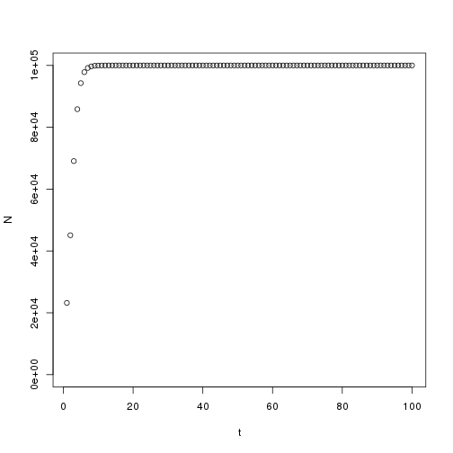
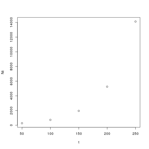
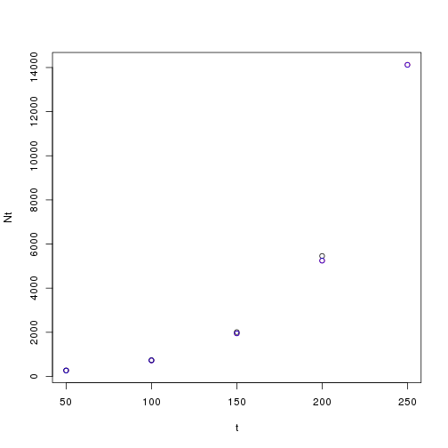
N0 <-100
r <- 0.02
t <- c(50, 100, 150, 200, 250)
ra <- log(1+r)
rb <- r
rc <- r -( (r^2)/2 )

Na <- N0*(exp(ra*t))
Nb <- N0*(exp(rb*t))
Nc <- N0*(exp(rc*t))

Na

[1] 269.1588 724.4646 1949.9603 5248.4897 14126.7721

Nb

[1] 271.8282 738.9056 2008.5537 5459.8150 14841.3159

Nc

[1] 269.1234 724.2743 1949.1920 5245.7326 14117.4964

plot(t, Na, col="red", ylab="Nt")
points( t, Nb, col="black")
points( t, Nc, col="blue")

$$\frac{dN}{[N(1-\frac{N}{K})]}=rdt$$


## Box C c

Given that:

$$\int \frac{1}{x(1+ax)} dx = ln \frac{x}{1+ax}$$

then:

$$\int_{N_0}^{N_t} \frac{1}{N(1- \frac{1}{K}N)} dN = ln \int_{t=0}^{t}r dt$$

Solve to get:

$$ln \frac{N_t}{1- \frac{1}{K} N_t} - ln \frac{N_0}{1- \frac{1}{K}N_0} = rt$$

ln(x) - ln(y) = ln(x/y) = ln(x*1/y)

$$ln \frac{N_t}{1- \frac{1}{K} N_t} . ln \frac{1- \frac{1}{K}N_0}{N_0} = rt$$

Inverse natural log of both sides:

$$\frac{N_t}{N_0} . \frac{1- \frac{1}{K}N_0}{1-\frac{1}{K}N_t} = e^{rt} $$

$$\frac{N_t - \frac{N_tN_0}{K}}{N_0 - \frac{N_tN_0}{K}} = e^{rt}$$

Multiply the left side by K/K

$$\frac{N_tK - N_tN_0}{N_0K - N_tN_0} = e^{rt}$$

$$\frac{N_t(K-N_0)}{N_0(K-N_t)} = e^{rt} $$

$$N_0e^{rt}(K-N_t) = N_t(K-N_0)$$

$$\frac{N_0e^{rt}}{K-N_0} = \frac{N_t}{K-N_t}$$


## Box C d
1
2
3
4
5
6
7
8
9
10
11
12
13
14
15
16
17
18
19
20
21
22
23
24
25
26
27
28
29
30
31
32
33

N.exact <- vector(mode="numeric", length=6)
N.exact[1] <- 1000
r <- 0.1
K <- 2000

for( t in 2:6){
N.exact[t] <- r*N.exact[t-1]*((K - N.exact[t-1])/K) + N.exact[t-1]
}

N.exact

[1] 1000.000 1050.000 1099.875 1149.376 1198.261 1246.295

N.approx <- vector(mode="numeric", length=6)
N.approx[1] <- 1000
C <- (K-N.approx[1])/N.approx[1]

for( t in 2:6){
N.approx[t] <- K/(1 + C*exp(-r*t))
}

N.approx

[1] 1000.000 1099.668 1148.885 1197.375 1244.919 1291.313


N.diff <- N.approx - N.exact

N.diff

[1] 0.00000 49.66799 49.01003 47.99907 46.65808 45.01739

## Box D preamble

With statistical software such as R, the manipulations described in Box D are unnecessary except to educate you as to what is going on behind the scenes. Here is one method to perform the manipulations as described in the box:

1
2
3
4
5
6
7
8
9
10
11
12
13
14
15
16
17
18
19
20
21
22
23
24
25
26
27
28
29
30
31
32
33
34
35
36
37
38
39
40
41
42
43
44
45
46
47
48
49
50
51
52
53
54
55
56
57
58
59
60
61
62
63
64
65
66
67
68
69
70
71
72
73
74
75
76
77
78
79
80
81
82
83
84
85
86
87
88
89
90
91
92
93
94
95
96
97
98
99
100
101
102
103
104
105
106
107
108
109
110
111
112
113
114
115
116
117
118
119
120
121
122
123
124
125
126
127
128
129
130
131
132
133
134
135
136
137
138
139
140
141
142
143
144
145
x <- c(1,2,3,4)
y <- c(3,7,6,9)

x.bar <- mean(x) # the mean of the X values
x.bar

[1] 2.5


y.bar <- mean(y) # the mean of the Y values
y.bar

[1] 6.25

x2.bar <- mean( x^2) # the mean of the X squared values
x2.bar

[1] 7.5

xy.bar <- mean( x*y ) #mean of the sum of the xy products
xy.bar

[1] 17.75

xy.cov <- xy.bar - (x.bar*y.bar) #covariance of x and y
xy.cov

[1] 2.125

x.var <- x2.bar - x.bar^2 # variance of x
x.var

[1] 1.25

m <- xy.cov/x.var # slope
m

[1] 1.7

b <- y.bar - m*x.bar # y intercept
b

[1] 2


# So the best fit line is y = mx + b or
# y = 1.7x + 2

# here is what you will normally do using R
# using the original x, y vectors from above

model <- lm(y~x)
summary(model)

Call:
lm(formula = y ~ x)

Residuals:
1 2 3 4
-0.7 1.6 -1.1 0.2

Coefficients:
Estimate Std. Error t value Pr(>|t|)
(Intercept) 2.0000 1.7958 1.114 0.381
x 1.7000 0.6557 2.592 0.122

Residual standard error: 1.466 on 2 degrees of freedom
Multiple R-squared: 0.7707, Adjusted R-squared: 0.656
F-statistic: 6.721 on 1 and 2 DF, p-value: 0.1221

##Now let's incorporate weights

x <- c(1,2,3,4)
y <- c(3,7,6,9)
w <- c(10,10,1,1)

w.sum <- sum(w) # sum of the weights
w.sum

[1] 22

xw.bar <- sum(x*w)/w.sum # the mean of the weighted X values
xw.bar

[1] 1.681818

yw.bar <- sum(y*w)/w.sum # the mean of the weighted Y values
yw.bar

[1] 5.227273

x2w.bar <- sum( x^2*w)/w.sum #mean of the sum of the weighted x squared values
x2w.bar

[1] 3.409091

xyw.bar <- sum( x*y*w )/w.sum #mean of the sum of the weighted xy products
xyw.bar

[1] 10.18182

xyw.cov <- xyw.bar - (xw.bar*yw.bar) #covariance of weighted x and y
xyw.cov

[1] 1.390496

xw.var <- x2w.bar - xw.bar^2 # variance of weighted x
xw.var

[1] 0.5805785

mw <- xyw.cov/xw.var # slope
mw

[1] 2.395018

bw <- yw.bar - mw*xw.bar # y intercept
bw

[1] 1.199288

# So the best fit line to the weighted data is y = mx + b or
# y = 2.4x + 1.2

# lm has a weight option

model <- lm(y~x, weight= w)
summary(model)

Call:
lm(formula = y ~ x, weights = w)

Weighted Residuals:
1 2 3 4
-1.879 3.196 -2.384 -1.779

Coefficients:
Estimate Std. Error t value Pr(>|t|)
(Intercept) 1.1993 1.7366 0.691 0.561
x 2.3950 0.9405 2.546 0.126

Residual standard error: 3.361 on 2 degrees of freedom
Multiple R-squared: 0.7643, Adjusted R-squared: 0.6464
F-statistic: 6.484 on 1 and 2 DF, p-value: 0.1258


## Box D a & b

Obtaining quantities 8 and 9 (slope and y intercept) for problems a and b is now trivial using the built in R function lm

1
2
3
4
5
6
7
8
9
10
11
12
13
14
15
16
17
18
19
20
21
22
23
24
25
26
27
28
29
30
31
32
33
34
35
36
37
38
39
40
41
42
43
44
45
46
47
48
49
x <- c(2,4,6,8)
y <- c(11,21,22,32)

model <- lm(y~x)
summary(model)

Call:
lm(formula = y ~ x)

Residuals:
1 2 3 4
-0.9 2.7 -2.7 0.9


Coefficients:
Estimate Std. Error t value Pr(>|t|)
(Intercept) 5.5000 3.4857 1.578 0.2553
x 3.2000 0.6364 5.028 0.0373 *
---
Signif. codes: 0 '***' 0.001 '**' 0.01 '*' 0.05 '.' 0.1 ' ' 1

Residual standard error: 2.846 on 2 degrees of freedom
Multiple R-squared: 0.9267, Adjusted R-squared: 0.89
F-statistic: 25.28 on 1 and 2 DF, p-value: 0.03735


w <- c(1,1,20,20)

model <- lm(y~x, weight= w)
summary(model)


Call:
lm(formula = y ~ x, weights = w)

Weighted Residuals:
1 2 3 4
4.021 5.913 -5.342 3.121

Coefficients:
Estimate Std. Error t value Pr(>|t|)
(Intercept) -1.1288 5.4466 -0.207 0.8550
x 4.0539 0.7854 5.162 0.0355 *
---
Signif. codes: 0 '***' 0.001 '**' 0.01 '*' 0.05 '.' 0.1 ' ' 1

Residual standard error: 6.686 on 2 degrees of freedom
Multiple R-squared: 0.9302, Adjusted R-squared: 0.8953
F-statistic: 26.64 on 1 and 2 DF, p-value: 0.03554

# Box E a $$0 = r_1N_1[ 1 - \frac{N_1 + \alpha_{21} N_2}{K_1} ]$$ $$0 = r_1N_1 - r_1N_1[\frac{N_1 + \alpha_{21} N_2}{K_1} ]$$ $$0 = r_1N_1 - \frac{r_1N_1N_1}{K_1} - \frac{r_1N_1 \alpha_{21} N_2}{K_1}$$ Subtract $r_1N_1$ from both sides and multiply by -1 $$r_1N_1= \frac{r_1N_1N_1}{K_1} + \frac{r_1N_1 \alpha_{21} N_2}{K_1}$$ Multiply by $\frac{K_1}{r_1N_1}$ $$K_1= N_1 + \alpha_{21} N_2$$ $$N_1= K_1 - \alpha_{21} N_2$$ Substitute for $N_1$ in $$0 = r_2N_2[ 1 - \frac{N_2 + \alpha_{12} N_1}{K_2} ]$$ $$0 = r_2N_2[ 1 - \frac{N_2 + \alpha_{12} (K_1 - \alpha_{21} N_2) }{K_2} ]$$ $$0 = r_2N_2 - r_2N_2[\frac{N_2 + \alpha_{12}K_1 - \alpha_{12}\alpha_{21} N_2 }{K_2} ]$$ $$0 = r_2N_2 + \frac{-r_2N_2N_2 - r_2N_2\alpha_{12}K_1 + r_2N_2\alpha_{12}\alpha_{21} N_2 }{K_2} $$ $$-r_2N_2K_2= -r_2N_2N_2 - r_2N_2\alpha_{12}K_1 + r_2N_2\alpha_{12}\alpha_{21} N_2$$ Divide by $-r_2N_2$
$$K_2= N_2 +\alpha_{12}K_1 - \alpha_{12}\alpha_{21} N_2$$ $$K_2 -\alpha_{12}K_1= N_2 - \alpha_{12}\alpha_{21} N_2$$ $$K_2 -\alpha_{12}K_1= N_2(1 - \alpha_{12}\alpha_{21})$$ $$\frac{K_2 -\alpha_{12}K_1}{1 - \alpha_{12}\alpha_{21}}= N_2$$
## Box E b
1
2
3
4
5
6
7
8
9
K1 <-1500
K2 <- 2500
a21 <- 0.25
a12 <- 0.5

N1 <- (K1-a21*K2)/(1-a21*a12)
N2 <- (K2-a12*K1)/(1-a21*a12)

cat( "The value of N1 is:", N1)
1
## The value of N1 is: 1000
1
cat( "The value of N2 is:", N2)
1
## The value of N2 is: 2000

$r_1$ and $r_2$ affect the rate of achieving equilibrium, not the final population count.

Share

Troop 272

Boy Scout Troop 272, Saint Joseph’s Parish, at Hidden Valley Scout Reservation, Gilmanton Iron Works, NH

1973

|||||||
|:—:|:—:|:—:|:—:|:—:|:—:|:—:|
|Back|Mr. McKinney|Mr. Davis|Mark Lovejoy||Jim Russo|Neil Duval|
|Third|Paul Desrocher|Paul McKiney|David Trask|Ed Hinton|Dennis Lavoie|?|
|Second|Bruce Badeau|Mark Lavoie||Ken Gifford|John Cloutier|Bill Courtemanche|
|Front|Jim Terriault|?|Joe Zulich|Peter LaPan|?|Mark Cote|

1974

1975

1976

Ed Hinton Ron Tetreault George Karageorge Mr. J. Bruce Davis Peter LaPan Joe Zulich Bill Courtemanche
Mark Lovejoy ? Ken Soares ? Steve Benson Tim Tetreault Jeff Greene
Tim Paiva ? Jim Stys Dennis Lavoie ? Ron Russo Rick Horne
? Mark Lavoie ?

1977

Back Bob Cormier Ron Tetreault Peter LaPan George Karageorge Bill Courtemanche
Middle Mike Horne Jim Stys Rick Horne Ron Russo Tom Lavoie Tim Paiva Dennis Lavoie
Front Alan Clarke Billy Lemire Roland Lavoie Jeff Greene Steve Benson Tim Tetreault Ken Soares

1978

Back Mark Lovejoy Paul Zeeley Tim Paiva George Karageorge Peter LaPan Bill Courtemanche Ed Hinton
Front Mike Zeeley Scott Turcotte Jim Rice Tim Tetreault Steve Benson Ron Russo Tom Lavoie
Share

troop272/hvsr1973

Saint Joseph's Parish, Nashua, NH Troop 272 at

Hidden Valley Scout Reservation

Gilmanton Ironworks, NH, 1973

Back Mr. McKiney Mr. Davis Jim Russo Neil Duval
Third Paul Desrocher Paul McKiney David Trask Mark Lovejoy Ed Hinton Dennis Lavoie ?
Second Bruce Badeau Mark Lavoie Ken Gifford John Cloutier Bill Courtemanche
Front Jim Terriault ? Joe Zulich Peter LaPan ? Mark Cote

Share

troop272/hvsr1974

Saint Joseph's Parish, Nashua, NH Troop 272 at

Hidden Valley Scout Reservation

Gilmanton Ironworks, NH, 1974

Back
Middle
Front

Share

troop272/hvsr1975

Saint Joseph's Parish, Nashua, NH Troop 272 at

Hidden Valley Scout Reservation

Gilmanton Ironworks, NH, 1975

Back
Middle
Front

Share