A couple of options for free, web based bibliography managers are Mendeley and Zotero. Given that Mendeley is owned by Elsevier, they are not an option. I started with Zotero, some configuration elements I will outline below, but eventually dropped them for Referencer. I like the idea of having complete control over my library. I am not interested in the “social” features of Zotero, I found upgrades to be difficult, and didn’t like the file structure utilized. Referencer is extremely simple, easy to install and configure, and gets the job done. I don’t anticipate many “upgrades” to the Referencer software - hopefully it will be maintained well into the future. I replicate the files to a cloud server for easy backup.

Referencer

#apt-get install referencer

Zotero

do not export, backup the database directory to retain metadata

~/.zotero/zotero/<3xdb….>/zotero…

the “pipes” subdir will not copy, be sure to compensate

pacman -S alsa-lib dbus-glib gcc-libs
pacman -S gtk2 nss #these were already installed

To configure the Zotero webdav server on Hostgator:

www.mysite.com/owncloud/remote.php/webdav ( /zotero automatically appended)
you will be prompted to create directory

Obtain street addresses

We would like to associate trees with street addresses when possible. When collecting tree data, we could also make note of the nearest address. Since we are collecting longitude/latitude data anyway, it would be convenient if we had a list of street addresses with associated longitude/latitude. This would allow us to auto-populate an address field based on longitude/latitude data. How does one obtain a list of all street addresses in town with longitude/latitude data? Let’s start with obtaining addresses alone. Addresses are availble commercially e.g. from the post office, but for a substantial fee. Since this is a volunteer effort, I want to see what I can get for free. Our town publishes property assessments on a regular basis, but this is hardcopy in the local paper. Though assessments are available online, it is through a query interface providing one at a time, with no obvious way to download the entire list. I was able to find our town’s street sweeping schedule which supplies a list of all streets in html format:

etc.

Copy paste into a text editor and with a little manipulation in R, I can get a vector of street names:

1
2
3
4
5
6
7
8
9
10
11

> rm(list=ls(all=TRUE))
> library(rjson)
> library(plyr)
>
> con <- file("streets-modified.csv", open="rt", encoding="latin1")
> all.streets <-unique( readLines(con))
> head(all.streets)
[1] "street"        "Aberdeen Rd "  "Academy St "   "Acton St "    
[5] "Adamian Park " "Adams St "    
> length(all.streets)
[1] 561

Looks like about 561 streets total. From my hardcopy assessment I learn that:

• Most streets don’t begin with 1 as the first address
• Addresses aren’t consecutive - there can be many gaps in numbering
• Most streets have fewer than 200 addresses
• A few of the main streets have up to 1600 addresses

Query for GPS coordinates

To obtain street addresses with lng/lat data I will use the DataScienceToolkit Google Style geocoder. To obtain coordinates I need to submit an address that looks like:

1 Aberdeen Road, Arlington, MA

This will return a data set that looks like:

[{“geometry”:{“viewport”:{“northeast”:{“lng”:-71.188745,”lat”:42.424604},”southwest”:{“lng”:-71.190745,”lat”:42.422604}},”location_type”:”ROOFTOP”,”location”:{“lng”:-71.189745,”lat”:42.423604}},”types”:[“street_address”],”address_components”:[{“types”:[“street_number”],”short_name”:”1”,”long_name”:”1”},{“types”:[“route”],”short_name”:”Aberdeen Rd”,”long_name”:”Aberdeen Rd”},{“types”:[“locality”,”political”],”short_name”:”Arlington”,”long_name”:”Arlington”},{“types”:[“administrative_area_level_1”,”political”],”short_name”:”MA”,”long_name”:”MA”},{“types”:[“country”,”political”],”short_name”:”US”,”long_name”:”United States”}],”formatted_address”:”1 Aberdeen Road Arlington MA”}]

You can see that lng= -71.188745 and lat=42.424604. I want to submit algorithmically, using a post to their URL. The post will look like:

“http://www.datasciencetoolkit.org/maps/api/geocode/json?sensor=false&address=1+Aberdeen+Rd+Arlington+MA“

I also want to count up the street addresses beginning at 1. This will give me a lng/lat for every address depending on how the geocoder handles addresses that don’t exist. Let’s find out.

1
2
3
4
5
6
7
8
9
10
11
12
13
14
15
16
17
18
19
20
21
22
23
24
25
26
27
28
29
30
31
32
33
34
35
36
37
38
39
40
41
42
43
44
45
46
47
48

> 
> 
> prefix <- 'http://www.datasciencetoolkit.org/maps/api/geocode/json?sensor=false&address='
> suffix <- "Arlington+MA"
> 
> arl.addresses <- data.frame( lng = numeric(), lat = numeric(), num=numeric(), street = character())
> 
> prefix <- 'http://www.datasciencetoolkit.org/maps/api/geocode/json?sensor=false&address='
> suffix <- "Arlington+MA"
> arl.addresses <- data.frame( lng = numeric(), lat = numeric(), num=numeric(), street = character())
> 
> for( i in 1:20){
+     middle <- gsub(" ","+",all.streets[10])
+     url <- paste( prefix, i, "+", middle, suffix, sep="")   #replace the space with a + sign
+     doc <- fromJSON(file=url, method='C')
+     arow <- data.frame( lng=doc$results[[1]]$geometry$location$lng,
+                        lat=doc$results[[1]]$geometry$location$lat,
+                        num=doc$results[[1]]$address_components[[1]]$short_name,
+                        street=doc$results[[1]]$address_components[[2]]$short_name)
+     
+     arl.addresses <- rbind(arl.addresses, arow)
+       
+   }
There were 20 warnings (use warnings() to see them)
> 
> arl.addresses
         lng      lat num   street
1  -71.14672 42.41162   1 Allen St
2  -71.14672 42.41162   2 Allen St
3  -71.14672 42.41151   3 Allen St
4  -71.14684 42.41160   4 Allen St
5  -71.14678 42.41145   5 Allen St
6  -71.14690 42.41153   6 Allen St
7  -71.14683 42.41139   7 Allen St
8  -71.14697 42.41146   8 Allen St
9  -71.14688 42.41132   9 Allen St
10 -71.14703 42.41139  10 Allen St
11 -71.14694 42.41126  11 Allen St
12 -71.14709 42.41132  12 Allen St
13 -71.14699 42.41120  13 Allen St
14 -71.14715 42.41125  14 Allen St
15 -71.14705 42.41114  15 Allen St
16 -71.14722 42.41118  16 Allen St
17 -71.14710 42.41108  17 Allen St
18 -71.14728 42.41110  18 Allen St
19 -71.14716 42.41102  19 Allen St
20 -71.14734 42.41103  20 Allen St
> 

Handling GPS data

1. Hardware
   
2. Software
   
3. Direct access to tty
   
4. Using gpsd
   

Hardware

Be sure to purchase a unit that will broadcast NMEA compliant sentences. I chose the Globalsat BU-353 shown below. This is a USB device that obtains power through the USB, but also has an internal battery for short term memory. Plug the unit into your laptop and allow a few minutes to get a fix. The led will start blinking once a fix has been obtained. You will not need any of the software provided with the unit.

Software

Guile 1.8 a dialect of Scheme/Lisp

gpsd a gps daemon. You will want to install the software compiled for your system, e.g. on Arch use

>pacman -S gpsd gpsd-clients

Direct access to tty

By default your gps unit is assigned to /dev/ttyUSB0, but you should check to make sure:

>dmesg | grep -i USB
[11250.384023] usb 4-2: new full-speed USB device number 2 using uhci_hcd
[11250.669968] usbcore: registered new interface driver usbserial
[11250.669991] USB Serial support registered for generic
[11250.670030] usbcore: registered new interface driver usbserial_generic
[11250.670033] usbserial: USB Serial Driver core
[11250.673280] USB Serial support registered for pl2303
[11250.685151] usb 4-2: pl2303 converter now attached to ttyUSB0
[11250.685174] usbcore: registered new interface driver pl2303
[11250.685177] pl2303: Prolific PL2303 USB to serial adaptor driver

Set access, change the baud rate and put the GPS in NMEA mode. Look at some of the output:

>sudo chmod 666 /dev/ttyUSB0 && stty -F /dev/ttyUSB0 ispeed 4800
>cat /dev/ttyUSB0
$GPGSA,A,3,15,14,09,18,21,24,22,06,19,,,,1.9,1.2,1.4*36
$GPGSV,3,1,12,18,71,317,34,24,63,112,31,21,52,212,28,15,42,058,34*71
$GPGSV,3,2,12,22,37,301,28,14,21,250,24,09,07,035,21,19,06,316,13*73
$GPGSV,3,3,12,06,05,279,18,26,01,060,,03,01,294,,28,01,024,*7F
$GPRMC,224355.000,A,1825.0332,N,02111.3093,W,0.13,134.34,050513,,,A*75
$GPGGA,224532.000,1825.0301,N,02111.3093,W,1,08,1.3,39.8,M,-73.7,M,,0000*25
$GPGSA,A,3,15,14,09,18,21,24,22,06,19,,,,1.9,1.2,1.4*36
$GPRMC,224356.000,A,4225.0330,N,02111.3093,W,0.33,145.51,050513,,,A*73
$GPGGA,224357.000,1825.0328,N,07111.3092,W,1,09,1.2,81.8,M,-33.7,M,,0000*5F
$GPGSA,A,3,15,14,09,18,21,24,22,06,19,,,,1.9,1.2,1.4*36
$GPRMC,224357.000,A,1825.0328,N,02111.3092,W,0.28,151.99,050513,,,A*71

Use Ctrl-C to stop the process.

Pick a sentence format that contains the coordinate information you wish to extract. I chose GPGGA.

>cat /dev/ttyUSB0 | grep GPGGA
$GPGGA,124532.000,1825.0301,N,02111.3093,W,1,08,1.3,39.8,M,-73.7,M,,0000*25
$GPGGA,124532.000,1825.0301,N,02111.3093,W,1,08,1.3,39.8,M,-73.7,M,,0000*25
$GPGGA,124532.000,1825.0301,N,02111.3093,W,1,08,1.3,39.8,M,-73.7,M,,0000*25
$GPGGA,124532.000,1825.0301,N,02111.3093,W,1,08,1.3,39.8,M,-73.7,M,,0000*25
$GPGGA,124532.000,1825.0301,N,02111.3093,W,1,08,1.3,39.8,M,-73.7,M,,0000*25
$GPGGA,124532.000,1825.0301,N,02111.3093,W,1,08,1.3,39.8,M,-73.7,M,,0000*25
$GPGGA,124532.000,1825.0301,N,02111.3093,W,1,08,1.3,39.8,M,-73.7,M,,0000*25
$GPGGA,124532.000,1825.0301,N,02111.3093,W,1,08,1.3,39.8,M,-73.7,M,,0000*25
$GPGGA,124532.000,1825.0301,N,02111.3093,W,1,08,1.3,39.8,M,-73.7,M,,0000*25
$GPGGA,124532.000,1825.0301,N,02111.3093,W,1,08,1.3,39.8,M,-73.7,M,,0000*25

You can extract to a text file using:

cat /dev/ttyUSB0 | grep --line-buffered   GPGGA > output.txt

Now with further munging you can extract the coordinates. I’ll save that for the next section where I use gpsd.

Using gpsd

Plug in your gps unit and start up gpsd. You will need to know the tty to which it is connected, see above.

gpsd -b  /dev/ttyUSB0

This launches the daemon which is now ready to be configured to accept requests. The “-b” switch means read only, to prevent writing that may lock up the unit. Use at your discretion. To verify the daemon is broadcasting, you can run either xgps (gui) or cgps, gpsmon (text) if you installed the client tools.

>gpsmon

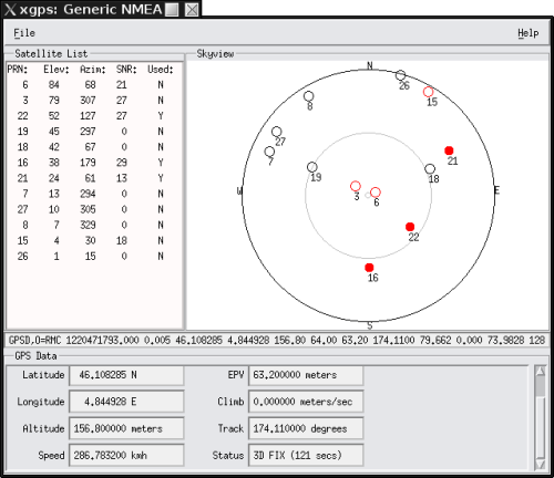
If everything is working you should see your coordinates displayed in the interface. Here is an example of what the xgps interface looks like:

Next we want to algorithmically extract coordinates from the daemon. Here I am using Guile. First I import two modules, rdelim which provides the read-line method, and srfi-1 which allows me to extract elements of a list using first, second, third, etc. Create a socket, connect the socket to port 2947 on my local machine and send the message "?WATCH={\"enable\":true,\"nmea\":true}" to indicate I am waiting for NMEA sentences.

(use-modules (ice-9 rdelim))
(use-modules (srfi srfi-1))

(define coords '())

(let ((s (socket PF_INET SOCK_STREAM 0)))
     (connect s AF_INET (inet-pton AF_INET "127.0.0.1") 2947)
     (send s "?WATCH={\"enable\":true,\"nmea\":true}")
     (do ((line  (read-line s) (read-line s)))
         ((string= (substring line 1 6) "GPGGA")
         (set! coords (list (third (string-split line #\,)) (fourth (string-split line #\,)) (fifth (string-split line #\,)) (sixth (string-split line #\,)))))))
 

I keep resetting the variable ‘line’ until I find a line that starts with GPGGA. Once obtained, I extract the coordinates and form a list which is named ‘coords’. Run the method to get the ouput below.

guile> guile> guile> guile> guile> ("4225.0384" "N" "78411.3104" "E")
guile> 

You now have a list of coordinates which can now be converted into the desired format.

I have used three Linux distributions: Ubuntu, Arch, and Debian. Here are my thoughts on the strengths and weaknesses of each.

Ubuntu

For a newcomer to Linux, Ubuntu is a natural choice. Canonical, the company behind Ubuntu, is a business, and as a business it is in their best interest to make Linux installation a no brainer. All drivers are included in the image and a live CD will allow you to experience Ubuntu without even installing the software. This allows you to determine if the distribution will work with your hardware, and test drive some of the applications. Once installed you will find all the features you expect from a mature desktop operating system. With a large user base, someone has probably already found a fix to problems you may experience.

Users migrating to Linux, myself included, are often migrating for the purpose of privacy and control. I don’t want to pay $1000 for a computer and then have to get Microsoft’s permission to use it. Meanwhile every keystroke is logged and my search queries a catalogued at headquarters. By signing up with Ubuntu, you are in for a similar experience. Desktop search pipes your queries to Amazon and the Ubuntu software manager will annoy you with advertisements for non-free crapware. Once you have become comfortable with Linux using Ubuntu, it is time to move on.

Arch

I thought I wanted a minimalist system, so I committed to Arch and the I3 window manager. Arch is a great system for someone who wants to learn Linux inside out. Nothing is preconfigured, forcing you to learn the intricasies of the configuration files. Most users will be hard core programmers - you have to be to deal with installation and configuration - so all problems have been encountered and solutions explicitly provided. I never had an Arch problem I couldn’t solve from reading the wiki. One quirk (feature?) of Arch is the rolling releases. When installing packages, you almost always need to run a system upgrade. 99% of the time this completes without problems, but occasionally, for example 2013-06-03 the file system directory layout was changed and a significant effort had to be invested in completing the upgrade. “Always read the Arch news before upgrading” - Arch is thoroughly and expertly documented, but this requires religious devotion.

The problem with Arch is that it requires a lot of work and time. Everything needs to be configured. For example, if you plug in a USB stick, nothing happens unless you configured auto-mount. I quickly came to realize that I don’t want to be a Linux guru, I just want to use Linux to get things done. That is what led me to Debian.

Debian

Debian is the distribution on which many other distributions (including Ubuntu) are built. Debian has the reputation for stability, with major releases occurring about every 2 years. Releases make use of well tested applications, sometimes a version or two behind what is currently available, to guarantee stability. Debian’s package manager is field tested and shared by many other distributions. Most software written for Linux will have an installation package for Debian. As I usually buy older computers with less memory, I use the minimalist Xfce window manager. Xfce has a clean layout, doesn’t install a lot of unnecessary software, yet provides the essentials you would expect in a modern window manager. There is a Debian installer that defaults to using Xfce as the window manager. I have been using Debian for a couple of years now and can report that I have encountered no issues that would prevent the average user from switching from Windows or Apple to Linux. The one exception would be Microsoft Office file compatibility. LibreOffice does a good job, but complex documents may not render properly.

Chapter 5 End Problems

Problem 2

1
2
3
4
5
6
7
8

condition <- letters[1:4]
N <- c(50,100, 50, 100)
Nm <- c(0.25, 0.5, 0.1, 0.2)
m <- Nm/N

d <- data.frame(condition,N,m)

plot(d$N, d$m, pch=as.character(d$condition))

Shifting balance favors smaller N and smaller m so C is the favored condition.

Problem 6

Start by setting r = x/ny to get the break even n. Anything larger is needed for altruistic behaviour to be favored by kin selection.

0.25 = 0.4/0.2n or n=0.4/(0.2*0.25) = 8 or greater

Problem 11

1
2
3
4
5
6
7
8
9
10
11
12
13
14

area <- c("dark","dark","light","light")
melanic <- c(T, F, T, F)
p.eaten <- c(0.26, 0.74, 0.86, 0.14)
p.survive <- 1-p.eaten

d <- data.frame(area, melanic, p.eaten, p.survive)
d2 <- split(d, area)

lapply(d2, function(x){ x[x$melanic==TRUE,"p.survive"]/x[x$melanic==FALSE,"p.survive"]  })  #melanic/nonmelanic survival ratio
## $dark
## [1] 2.846154
## 
## $light
## [1] 0.1627907

Problem 14

1
2
3
4
5
6
7
8
9
10
11
12
13
14
15
16
17
18
19

J.1 <- c(0.12, 0.8, 0.06, 0.02)

J.2 <- c(0.3,0.56, 0.1, 0.04)

J.11 <- sum(J.1^2)
J.11
## [1] 0.6584
J.22 <- sum(J.2^2)
J.22
## [1] 0.4152
J.12 <- sum(J.1*J.2)
J.12
## [1] 0.4908
I <- J.12/sqrt(J.11*J.22)  #from p408
I
## [1] 0.938709
D <- -log(I)
D
## [1] 0.06324978

Problem 15

1
2
3
4
5
6
7
8
9
10
11
12
13
14
15
16
17
18
19

J.1 <- c(0.3, 0.5)

J.2 <- c(0.2, 0.3)

J.11 <- sum(J.1^2)
J.11
## [1] 0.34
J.22 <- sum(J.2^2)
J.22
## [1] 0.13
J.12 <- sum(J.1*J.2)
J.12
## [1] 0.21
I <- J.12/sqrt(J.11*J.22)  #from p408
I
## [1] 0.9988681
D <- -log(I)
D
## [1] 0.001132503

eStudio is a Java applet that runs in a browser. eStudio can be used to display a continuous loop of images on any computer with a browser. The features of eStudio are:

• Display a continuous cycle of images. Image number is limited by available RAM
• Images are grouped by categories, one category per subdirectory
• Customize to use your own images
• Optional annotation can be displayed with the image
• Working example provided
• Turn a laptop into a "kiosk" style display
• Runs in any browser equipped with Java 1.4 or higher plug-in
• Currently works on Windows only

Installation

1. Create an installation directory on your hard drive.
2. Download eStudio.zip into the installation directory. Unzip
3. Click on start.html to launch the applet.
4. Click on customize.html for customization information.

Chapter 5 Box Problems

Box A

(a)

$$\displaystyle W_{BB}=p^2_1(1-2 \alpha + 2 \epsilon) + 2p_1q_1(1-\alpha+\epsilon) + q^2_1$$

$$ = p^2_1 - 2p^2_1 \alpha + 2p^2_1 \epsilon + 2p_1q_1 - 2p_1q_1 \alpha + q^2_1 + 2p_1q_1 \epsilon$$

$$\displaystyle = p^2_1 - 2p_1q_1 + q^2_1 + 2p_1[ -p_1 \alpha + p_1 \epsilon - q_1 \alpha + q_1 \epsilon]$$

$$\displaystyle = (p+q)^2 + 2p_1[ -\alpha + p_1 \epsilon]$$

$$\displaystyle = 1 - 2p_1[p_1 \alpha - p_1\epsilon + q_1 \alpha - q_1 \epsilon]$$

$$\displaystyle = 1 - 2p_1[(p_1+q_1)\alpha - (p_1+q_1)\epsilon]$$

$$\displaystyle = 1 - 2p_1( \alpha - \epsilon)$$

(b)

$$\displaystyle W_{Bb} = p^2_1 (1-\alpha+2\epsilon) + 2p_1q_1(1+ \epsilon) +q^2_1(1-\alpha)$$

$$\displaystyle = p^2_1 -p^2_1\alpha+2p^2_1\epsilon + 2p_1q_1 + 2p_1q_1\epsilon +q^2_1 - q^2_1\alpha$$

$$\displaystyle = p^2_1 + 2p_1q_1 +q^2_1 -(p^2_1\alpha +q^2_1\alpha)+2p^2_1\epsilon + 2p_1q_1\epsilon$$

$$\displaystyle = 1-\alpha(p^2+q^2) + 2p_1\epsilon(p_1+q_1)$$

$$\displaystyle = 1-(p^2+q^2)\alpha + 2p_1\epsilon$$

(c)

$$\displaystyle W_{bb} = p^2_1(1+2\epsilon)+2p_1q_1(1-\alpha+\epsilon)+q^2_1(1-2\alpha)$$

$$\displaystyle = p^2_1 +2p^2_1\epsilon +2p_1q_1 - 2p_1q_1\alpha + 2p_1q_1\epsilon +q^2_1 -2q^2_1\alpha$$

$$\displaystyle = p^2_1 + 2p_1q_1 +q^2_1 + 2p^2_1\epsilon + 2p_1q_1\epsilon - 2p_1q_1\alpha - 2q^2_1\alpha$$

$$\displaystyle = 1 + 2p_1\epsilon(p_1+q_1) - 2q_1\alpha(p_1+q_1)$$

$$\displaystyle = 1 +2p_1\epsilon -2q_1\alpha$$

(d)

Extract expressions for alpha and epsilon from Table 1 page 330

$$\displaystyle W_{AA}=p^2_2(1-2\alpha+2\epsilon)+2p_2q_2(1-\alpha+2\epsilon)+q^2_2(1+2\epsilon)$$

$$\displaystyle = p^2_2 - p^2_2\alpha + p^2_2\epsilon + 2p_2q_2 - 2p_2q_2\alpha + 4p_2q_2\epsilon + q^2_2 +2q^2_2\epsilon$$

$$\displaystyle = p^2_2 + 2p_2q_2 +q^2_2 +2\epsilon(p^2_2 + 2p_2q_2 +q^2_2)-2p_2\alpha(p_2+q_2)$$

$$\displaystyle = 1+2\epsilon - 2p_2\alpha$$

(e)

$$\displaystyle W_{Aa}= p^2_2(1-\alpha+\epsilon)+2p_2q_2(1+\epsilon)+q^2_2(1-\alpha+\epsilon)$$

$$\displaystyle = p^2_2 -p^2_2\alpha +p^2_2\epsilon +2p_2q_2 +2p_2q_2\epsilon+ q^2_2 - q^2_2\alpha + q^2_2\epsilon$$

$$\displaystyle = p^2_2 + 2p_2q_2 + q^2_2 + \epsilon(p^2_2 + 2p_2q_2 + q^2_2)-\alpha(p^2_2-q^2_2)$$

$$\displaystyle = 1 + \epsilon - \alpha(p^2_2+q^2_2)$$

(f)

$$\displaystyle W_{aa}= p^2_2(1) + 2p_2q_2(1-\alpha)+q^2_2(1-2\alpha)$$

$$\displaystyle = p^2_2 + 2p_2q_2 - 2p_2q_2\alpha + q^2_2 - 2q^2_2\alpha$$

$$\displaystyle = p^2_2 + 2p_2q_2 + q^2_2 - 2q_2\alpha(p_2+q_2)$$

$$\displaystyle = 1-2q_2\alpha$$

(g)

$$\displaystyle = p^2_2[1-2p_1(\alpha-\epsilon)]+2p_2q_2[1-(p^2_1+q^2_1)\alpha+2p_1\epsilon]+q^2_2(1-2q_1\alpha+2p_1\epsilon)$$

$$\displaystyle = p^2_2-2p_1p^2_2(\alpha-\epsilon)+2p_2q_2-2p_2q_2(p^2_1+q^2_1)\alpha + 2p_1p_2q_2\epsilon+q^2_2-2q_1q^2_2\alpha+2p_1q^2_2\epsilon$$

$$\displaystyle = p^2_2-2p_1p^2_2\alpha + 2p_1p^2_2\epsilon +2p_2q_2-2p^2_1p_2q_2\alpha - 2p_2q^2_1q_2\alpha+2p_1p_2q_2\epsilon + q^2_2-2q_1q^2_2\alpha+2p_1q^2_2\epsilon$$

Rearrange into 3 sections collecting similar variables


Section 1 - terms without alpha or epsilon:

$$\displaystyle = p^2_2 + 2p_2q_2 + q^2 = 1$$

Section 2 - terms with alpha:

$$\displaystyle = -2p_1p^2_2\alpha - 2p^2_1p_2q_2\alpha-2p_2q^2_1q_2\alpha-2q_1q^2_2\alpha$$

$$\displaystyle = -2\alpha[p_1p^2_2+p^2_1p_2q_2+p_2q^2_1q_2+q_1q^2_2]$$

$$\displaystyle = -2\alpha[ p_1p_2(p_2+p_1q_2)+q_1q_2(q_1p_2+q_2)]$$

Substitute \(p_1=1-q_1\) and \(q_1=1-p_1\)

$$\displaystyle = -2\alpha[p_1p_2(p_2+(1-q_1)q_2)+q_1q_2((1-p_1)p_2+q_2) ]$$

$$\displaystyle = -2\alpha[p_1p_2(p_2+q_2-q_1q_2)+ q_1q_2(p_2-p_1p_2+q_2) ]$$

$$\displaystyle = -2\alpha[p_1p_2(1-q_1q_2)+q_1q_2(1-p_1p_2)]$$

$$\displaystyle = -2\alpha[p_1p_2-p_1p_2q_1q_2+q_1q_2-p_1p_2q_1q_2]$$

$$\displaystyle = -2\alpha[p_1p_2+q_1q_2-2p_1p_2q_1q_2]$$

Substitute \(q_1=1-p_1\) and \( q_2=1-p_2\)

$$\displaystyle = -2\alpha[ p_1p_2+(1-p_1)(1-p_2)-2p_1p_2(1-p_1)(1-p_2)]$$

$$\displaystyle = -2\alpha[ p_1p_2 + 1-p_1-p_2+p_1p_2-2p_1p_2(1-p_1-p_2+p_1p_2)]$$

$$\displaystyle = -2\alpha[p_1p_2 + 1-p_1-p_2 +p_1p_2 -2p_1p_2+2p_1p^2_2+2p^2_1p_2-2p^2_1p^2_2 ]$$

$$\displaystyle = -2\alpha[1-p_1-p_2+2p_1p_2(p_1+p_2-p_1p_2) ]$$

Section 3 - terms with epsilon:

$$\displaystyle = 2p_1p^2_2\epsilon + 2p_1p_2q_2\epsilon + 2p_1q^2_2\epsilon=2p_1\epsilon(p^2_2+p_2q_2 + q^2_2)=2p_1\epsilon$$

So finally \(\bar{w} = 1 -2\alpha[1-p_1-p_2+2p_1p_2(p_1+p_2-p_1p_2) ] +2p_1\epsilon\)

Box B

From chapter 4 Box E p269 The fundamental theorum of natural selection:

$$\displaystyle i_w=\frac{\sigma_w}{\bar{w}}$$

From chapter 4 Box B p258

$$\displaystyle \Delta p = \frac{i_wpq\alpha_w}{\sigma_w}$$

Substitute to get: \(\Delta p=\frac{pq\alpha_w}{\bar{w}}\)

For x changing in response to selection: \(\Delta p=\frac{i_xpq\alpha_x}{\sigma_x}\)

Set the 2 equations for \(\Delta p\) equal and solve for \(i_x\)

From chapter 1 Box E part b:

1
2
3
4
5
6
7
8
9
10
11
12
13
14
15
16
17

K1 <- 1500  #population of interest
K2 <- 2500  #competitor population
alpha21 <- 0.25
alpha12 <- 0.5
N1 <- 1000
N2 <- 2000
r <- 0.05

#equation 1
1-(N1 + alpha21*N2)/K1
## [1] 0
#equation 2
r*(N1+alpha21*N2)/K1^2
## [1] 3.333333e-05
#equation 3
-r*N2/K1
## [1] -0.06666667

Box C

$$\displaystyle r=2F_{IR}$$

Box D

Only q can be calculated from the nonmelanic (aa freq=q^2) phenotype so take the melanic frequencies and subtrac from one.

Calculate p as 1-q

For Biston betularia:

1
2
3
4
5
6
7
8
9
10
11
12
13
14
15
16
17
18
19
20
21

q0 <- sqrt(0.99)

q0
## [1] 0.9949874

p0 <- 1- q0  
p0
## [1] 0.005012563

qt <- sqrt(0.05)
qt
## [1] 0.2236068
pt <- 1- qt
pt
## [1] 0.7763932
N <- 50
N
## [1] 50
s <- (1/N)*(log((pt*q0)/(p0*qt)) + 1/qt - 1/q0)
s
## [1] 0.200053

For Biston cognitaria:

1
2
3
4
5
6
7
8
9
10
11
12
13
14
15
16
17
18
19
20
21
22
23
24

q0 <- sqrt(0.99)
q0
## [1] 0.9949874

p0 <- 1- q0  
p0
## [1] 0.005012563

qt <- sqrt(0.20)
qt
## [1] 0.4472136

pt <- 1- qt
pt
## [1] 0.5527864

N <- 30
N
## [1] 30

s <- (1/N)*(log((pt*q0)/(p0*qt)) + 1/qt - 1/q0)
s
## [1] 0.2244583

Box E

(a)

For Biston betularia:

1
2
3
4
5

p0 <- 0.005
pt <- 0.776
C <- log(pt) - log(p0)
C
## [1] 5.044715

For Biston cognitaria:

1
2
3
4
5

p0 <- 0.01
pt <- 0.553	
C <- log(pt) - log(p0)
C
## [1] 4.012773

(b)

Given: $$\displaystyle \frac{dp}{dt}=\frac{pqs}{2\bar{w}}$$ rearrange to $$\displaystyle\frac{sq}{\bar{w}}dt=\frac{2}{p}dp$$

Given: $$\displaystyle C=\int^t_0 \frac{sq}{\bar{w}}dt$$ substitute to get $$\displaystyle C=\int^t_0 \frac{2}{p}dp = 2\int^t_0\frac{1}{p}dp=2ln(p_t)-2ln(p_0)=2[ln(p_t)-ln(p_0)]$$

(c)

Given: $$\displaystyle \frac{dp}{dt}=\frac{p^2qs}{\bar{w}}$$ rearrange to $$\displaystyle\frac{sq}{\bar{w}}dt=\frac{1}{p^2}dp$$

Given: \(\displaystyle C=\int^t_0\frac{sq(1+p)}{\bar{w}}dt=\int^t_0(1+p)\frac{sq}{\bar{w}}dt\) substitute to get

$$C=\int^t_0 \frac{(1+p)}{p^2}dp = |^t_0 -\frac{1}{p}+ln(p) = -\frac{1}{p_t}+ln(p_t)+\frac{1}{p_0}-ln(p_0)$$

(d)

1
2
3
4
5
6
7
8
9
10
11
12
13
14
15
16
17

pt <- 1
p0 <- 0.01

log(pt)-log(p0)     #dominant
## [1] 4.60517
-(1+log(p0)-(1/p0)) #recessive
## [1] 103.6052
-2*log(p0)          # additive
## [1] 9.21034
p0 <- 0.001

log(pt)-log(p0)     #dominant
## [1] 6.907755
-(1+log(p0)-(1/p0)) #recessive
## [1] 1005.908
-2*log(p0)          # additive
## [1] 13.81551

(e)

For 10% selective elimination B = 0.9 (fraction retained for breeding) and the corresponding i is 0.195 (Box C chpt 4).

1
2
3
4
5
6
7
8
9
10
11
12

i <- 0.195
t <- 1    #(per generation)

n <- 10
(i/3.14159276)*sqrt(n/2)
## [1] 0.1387937
n <- 30
(i/3.14159276)*sqrt(n/2)
## [1] 0.2403977
n <- 100
(i/3.14159276)*sqrt(n/2)
## [1] 0.4389042

(f)

1
2
3
4
5
6
7
8
9
10
11
12
13
14
15

subpop <- c(1,1,1,2,2,3,3)
deme <- c(1,2,3,1,2,1,2)
p <- c(0.9,0.8,0.7,0.6,0.5,0.4,0.3)
H <- c(0.18,0.32,0.42,0.48,0.50,0.48,0.42)
p2 <- p^2
d <- data.frame(cbind(subpop,deme,p,p2,H))
d
##   subpop deme   p   p2    H
## 1      1    1 0.9 0.81 0.18
## 2      1    2 0.8 0.64 0.32
## 3      1    3 0.7 0.49 0.42
## 4      2    1 0.6 0.36 0.48
## 5      2    2 0.5 0.25 0.50
## 6      3    1 0.4 0.16 0.48
## 7      3    2 0.3 0.09 0.42

1
2
3
4
5
6
7
8
9
10
11
12
13
14
15
16
17
18
19
20
21
22
23
24
25
26
27
28
29
30
31
32
33
34
35
36
37
38
39
40
41
42
43
44
45
46
47
48
49

#Calculate each summary statistic using dplyr's group_by function

Sp <- (group_by(d, subpop) %>% summarize(sum(p)))[,2] #sum of p within subpopulation
n <- (group_by(d, subpop) %>% summarize(length(p)))[,2] #count
p.bar <- (group_by(d, subpop) %>% summarize(mean(p)))[,2] #mean p
Sp2 <- (group_by(d, subpop) %>% summarize(sum(p2)))[,2] #sum p squared

H.bar <- (group_by(d, subpop) %>% summarize(mean(H)))[,2] #mean H
d2 <- data.frame( c(Sp, n, p.bar, H.bar, Sp2))
names(d2) <- c("Sp", "n", "p.bar", "H.bar","Sp2")
np.bar2 <- d2$n*d2$p.bar^2

d2 <- cbind(d2, np.bar2)

d2

##    Sp n p.bar     H.bar  Sp2 np.bar2
## 1 2.4 3  0.80 0.3066667 1.94   1.920
## 2 1.1 2  0.55 0.4900000 0.61   0.605
## 3 0.7 2  0.35 0.4500000 0.25   0.245

TSS <- sum(d2$Sp2) - sum(d2$n)*(mean(d2$p.bar)^2)
TSS

## [1] 0.5522222

BSS <- sum(d2$n*d2$p.bar^2) - sum(d2$n)*(mean(d2$p.bar)^2)
BSS
## [1] 0.5222222


WSS <- TSS - BSS
WSS
## [1] 0.03

sigma2.DS <- WSS/sum(d2$n)
sigma2.DS

## [1] 0.004285714

sigma2.ST <- BSS/sum(d2$n)
sigma2.ST

## [1] 0.07460317

sigma2.DT <- TSS/sum(d2$n)
sigma2.DT

## [1] 0.07888889

(a)

1
2
3
4
5
6
7
8
9
10
11
12
13
14
15
16
17
18
19
20
21
22
23

d3 <- split(d, subpop)

variances <- lapply(d3, function(x){  (x$p-mean(x$p))^2    })
variances
## $`1`
## [1] 0.01 0.00 0.01
## 
## $`2`
## [1] 0.0025 0.0025
## 
## $`3`
## [1] 0.0025 0.0025
variances.avg <- sapply(variances, function(x){  mean(x)    }) #averages
variances.avg
##           1           2           3 
## 0.006666667 0.002500000 0.002500000
variances.n <- sapply(variances, function(x){ length(x)}) #counts per subpopulation
variances.n
## 1 2 3 
## 3 2 2
avg.weighted.variance <- sum(variances.avg*variances.n)/sum(variances.n )
avg.weighted.variance
## [1] 0.004285714

(b)

1
2

sum(((d2$p.bar - mean(d2$p.bar))^2)*d2$n)/sum(d2$n)
## [1] 0.0368254

(c)

1
2

sum((d$p - mean(d$p))^2)/length(d$p)
## [1] 0.04

(d)

1
2
3
4
5
6
7
8
9
10
11
12
13
14
15
16
17
18
19

H.D <- sum(d$H)/nrow(d)
H.D
## [1] 0.4
H.variances.avg <- sapply(d3, function(x){ mean(x$H) }) #H averages
H.variances.avg
##         1         2         3 
## 0.3066667 0.4900000 0.4500000
H.S <- sum(H.variances.avg*variances.n)/nrow(d)
H.S
## [1] 0.4
H.T <- 2*mean(d$H)*(1-mean(d$H))  #see part c 
H.T
## [1] 0.48
H.S - H.D
## [1] 0
H.T - H.S
## [1] 0.08
H.T - H.D
## [1] 0.08

(e)

1
2
3
4
5
6
7
8
9
10
11
12
13

F.DS <- (H.S-H.D)/H.S
F.DS
## [1] 0
F.ST <- (H.T-H.S)/H.T
F.ST
## [1] 0.1666667
F.DT <- (H.T-H.D)/H.T
F.DT
## [1] 0.1666667
(1-F.DS)*(1-F.ST)
## [1] 0.8333333
(1-F.DT)
## [1] 0.8333333

(f)

I will call the quantity \(\displaystyle \frac{\Sigma n_i\bar{p}_i(1-\bar{p}_i)}{\Sigma n_i}\) “tilde.pq” in the R code.

1
2
3
4
5
6
7
8
9
10
11
12
13
14

tilde.pq <- sum(d2$n*d2$p.bar*(1-d2$p.bar))/sum(d2$n)

tilde.pq
## [1] 0.2042857

sigma2.DS/tilde.pq
## [1] 0.02097902

sigma2.ST/tilde.pq
## [1] 0.3651904

sigma2.DT/tilde.pq
## [1] 0.3861694

##Compare parental and mutant sequences

After perfoming error prone PCR (random) or oligonucleotide (directed) mutagenesis you will want to visualize your sequences and determine the rate of mutation incorporation. A typical visualization is the stacked bar chart as in this figure from Finlay et al. JMB (2009) 388, 541-558:

To decode this graphic you must:

• estimate the percentage of each amino acid by comparison to the Y axis
• compare relative amino acid abundance by comparing the area of boxes
• correlate color with amino acid identity
• compare to the reference sequence at the bottom of the graph

An easier to interpret graphic would be a scatter plot of sequence index (i.e. nucleotide position) on the X axis vs frequency on the Y. The data points are the single letter amino acid code. Highlight the reference sequence with a red letter.

The first step is to align all sequences. Start with a multi-fasta file of all sequences:

$cat ./myseqs.fasta

>ref
GLVQXGGSXRLSCAASGFTFSSYAMSWVRQAPGKGLEWVSAISGSGGSTYY
ADSVKGRFTISRDNSKNTLYLQMNSLRAEDTAVYYCAKDHRRPKGAFDIWGQGTMVTVSS
GGGGSGGGGSGGGGSGQSALTQPASVSGSPGQSITISCTGTSSDVGAYNYVSWYQQYPGK
APKLMIYEVTNRPSGVSDRFSGSKSGNTASLTISGLQTGDEADYYCGTWDSSLSAVV
>BSA130618a-A01
glvxxggxxrlscasgftfssyamswvrqapgklewvsaisgsggstyysdsvkgrftissdnskntlylqmnslraedt
avyycakdhrrpkgafdiwgqgtmvtvssggggsggggsggggsgqsaltqprsvsgtpgqsviisctgtssdvggskyv
swyqqhpgnapkliiydvserpsgvsnrfsgsksgtsaslaitglqaedeadyycqsydsslvvf
>BSA130618a-A02
glvqpggxxrlscasgftfssyamswvrqapgkglewvsaisgsggstyyadsvkgrftisrdnskntlylqmnslraed
tavyycakdhrrpngafdiwgqgtmvtvssggggsggggsggggsgqsvvtqppsmsaapgqkvtiscsgsssnignnyv
swyqqlpgtapklliydnnkrpsxipdrfsgsksgtsatlitglqtgdeadyycgtwdsslsagvf
>BSA130618a-A03
glvqxggxxrlscasgftfssyamswvrqapgkglewvsaisgsggstyyadsvkgrftisrdnskntlylqmnslraed
tavyycakdhrrpkgafdiwgqgtmvtvssggggsggggsggggsgsyeltqppsvsvspgqtasitcsgsssniginyv
swyqqvpgtapklliyddtnrpsgisdrfsgsksgtsatlgitglqtgdeadyycgtwdsslsvvvf

Above I have labeled my parental reference sequence “ref”. Use clustalo to perform the alignment and request the output in “clustal” format. The clustalo command can be run from within R using the system command. Read the alignment file into a matrix:

  input.file <- paste( getwd(), "/out.fasta", sep="")
  output.file <-  paste( getwd(), "/out.aln", sep="")
  system( paste("c:/progra~1/clustalo/clustalo.exe -infile=", input.file, " -o ", output.file, ".aln --outfmt=clustal", sep=""))   
 
 in.file <- paste(getwd(), "/out.aln", sep="")	
 seqs.aln <- as.matrix(read.alignment(file = in.file, format="clustal"))

At each position determine the frequency of all 20 amino acids. Set up
a second matrix that has one dimension as the length of the sequence
and the other as 20 for each amino acid. This is the matrix that will
hold the amino acid frequencies.

The R package “seqinr” provides a constant containing all single character amino acids as well as asterisk for the stop codon. Use this to name the rows of the frequency matrix.

      library(seqinr)
levels(SEQINR.UTIL$CODON.AA$L)

[1] "*" "A" "C" "D" "E" "F" "G" "H" "I" "K" "L" "M" "N" "P" "Q" "R" "S" "T" "V"
[20] "W" "Y"

aas <- c(levels(SEQINR.UTIL$CODON.AA$L), 'X')
freqs <- matrix(  ncol=dim(seqs.aln)[2], nrow=length(aas))
rownames(freqs) <- aas

#Process through the matrix, calculating the frequency for each amino acid.
for( col in 1:dim(aligns)[2]){
     for( row in 1:length(aas)){
        	  freqs[row, col] <- length(which(toupper(seqs.aln[,col])==aas[row]))/dim(seqs.aln)[1]
        }
}

Set up an empty plot for Frequency (Y axis) vs nucleotide index (X axis).
Y range is 0 to 1, X range is one to the length of the sequence i.e. the number of columns in the frequency matrix.
Plot frequencies >0 in black, using the single letter amino acid code as the plot character.

     plot(1, type="n", xlab="Sequence Index", ylab="Frequency", xlim=c(1, dim(freqs)[2]), ylim=c(0, 1))
for( i in 1:length(aas)){
         points( which(freqs[i,]>0), freqs[i, freqs[i,]>0], pch=rownames(freqs)[i], cex=0.5)
       }

Overlay the reference sequence in red.

ref <-seqs.aln[rownames(seqs.aln)=="ref",]
for(i in 1:length(ref)){
       if(  length( freqs[rownames(freqs)[rownames(freqs)==toupper(ref[i])],i] ) > 0){
    if(freqs[rownames(freqs)[rownames(freqs)==toupper(ref[i])],i] > 0){
                    points( i,freqs[rownames(freqs)[rownames(freqs)==toupper(ref[i])],i]  , pch=toupper(ref[i]), cex=0.5, col="red")
              }
       	    }
    }

This is what it looks like (open in a new tab to see detail):

It’s easy to see which amino acid is parental, and its relative abundance to other amino acids is clear.
Consider position 61: N is the parental amino acid but T is now more abundant in the panel of mutants. K and S are the next most abundant amino acids.

Should multiple amino acids have the same or close to the same frequency, the graph can get cluttered and difficult to interpret. Adjusting the Y axis can help clarify amino acid identity. At each position percentages may not add up to 100 depending on the number of gaps. Consider the sequence “RFSGS” at positions 69-73 which is in a region containing gaps for some of the clones:

Chapter 4 End Problems

Problem 1

1
2
3
4
5
6
7
8

u <- 80
u.s <- 110
u.prime <- 90
S <- u.s - u  #selection differential
R <- u.prime - u  # response to selection
h2 <- R/S  #realized heritability
h2
## [1] 0.3333333

Problem 2

1
2
3
4
5
6
7
8

u <- 140
u.s <- 165
h2 <- 0.4
S <- u.s - u  #selection differential
R <- h2*S
u.prime <- u + R
u.prime
## [1] 150

If females only have u.s=165 and we assume males u=140 then the average u.s = (165+140)/2 = 152.5

1
2
3
4
5
6
7
8

u <- 140
u.s <- 152.5 
h2 <- 0.4
S <- u.s - u  #selection differential
R <- h2*S
u.prime <- u + R
u.prime
## [1] 145

Problem 3

1
2
3
4
5
6
7
8

u <- 60
u.s <- 48
h2 <- 0.12
S <- u.s - u  #selection differential
R <- h2*S
u.prime <- u + R
u.prime
## [1] 58.56

Problem 4

1
2
3
4
5
6
7
8
9
10
11
12
13
14
15
16
17
18

u.s <- 35
u.prime <- 25 
h2 <- 0.4


#S <- u.s - u  #selection differential
#R <- h2*S
#u.prime <- u + R  or R <- u.prime - u

#Rearrange to get:

#R <- h2*(u.s-u)
#u.prime - u <- h2*(u.s-u)
#solve for u:

u <- (u.prime-h2*u.s)/(1-h2)
u
## [1] 18.33333

Problem 5

1
2
3
4
5
6
7
8
9
10
11
12
13

u <- 110
h2 <- 0.25
#S <- u.s - u  #selection differential
S <- 80
u.s <- S + u
u.s
## [1] 190
R <- h2*S
R
## [1] 20
u.prime <- u + R
u.prime
## [1] 130

Problem 6

1
2
3
4
5
6
7
8
9
10
11
12
13
14
15
16
17
18
19

u <- 100
#S <- u.s - u  #selection differential
S <- 32
u.s <- S + u
u.s
## [1] 132
#From Table IX p292 half sib covariance equals the additive genetic variance divided by 4 so

sigma2.a <- 12*4
sigma2.p <- 240
h2 <- sigma2.a/sigma2.p
h2
## [1] 0.2
R <- h2*S
R
## [1] 6.4
u.prime <- u + R  
u.prime 
## [1] 106.4

Problem 7

$$\displaystyle\sigma^2_g + \sigma^2_e = 240$$

$$\displaystyle\sigma^2_e = 90$$ so

$$\displaystyle\sigma^2_g = 240 - 190 = 50$$

Broad sense heritability =
$$\displaystyle\frac{ \sigma^2_g }{ \sigma^2_g + \sigma^2_e } = \frac{50}{240} = 0.208$$

Problem 8

Broad sense heritability $$\displaystyle h^2= \frac{\sigma^2_g}{\sigma^2_p} = \frac{\sigma^2_a +\sigma^2_d +\sigma^2_i }{\sigma^2_p} = 0.7$$

Narrow sense heritability $$\displaystyle h^2= \frac{\sigma^2_a}{\sigma^2_p}$$

If $$\displaystyle \sigma^2_d +\sigma^2_i = 0$$ then Broad sense heritability and narrow sense heritability are the same and so the maximum narrow sense is 0.7. Heritability can be zero, so the range is 0 - 0.7.

Problem 9

Narrow sense heritability $$\displaystyle h^2= \frac{\sigma^2_a}{\sigma^2_p}$$

Rearrange: $$\displaystyle \sigma^2_a = h^2\sigma^2_p$$

Jones: 0.24 x 4= 0.96 = $$\displaystyle\sigma^2_a$$

Smith: 0.12 x 4 = 0.48 = $$\displaystyle\sigma^2_a$$

Problem 10

1
2
3
4
5
6
7
8
9
10
11
12
13
14
15
16
17
18
19
20
21
22
23
24

x <- c(21, 15, 9)
y <- log(x)
y
## [1] 3.044522 2.708050 2.197225
u.x.asterisk <- (x[1] + x[3])/2
a.x <- x[1] - u.x.asterisk
d.x <- x[2] - u.x.asterisk

 u.x.asterisk; a.x; d.x;
## [1] 15
## [1] 6
## [1] 0
u.y.asterisk <- (y[1] + y[3])/2
a.y <- y[1] - u.y.asterisk
d.y <- y[2] - u.y.asterisk

u.y.asterisk; a.y; d.y;
## [1] 2.620874
## [1] 0.4236489
## [1] 0.08717669
exp(u.y.asterisk); exp(a.y); exp(d.y);
## [1] 13.74773
## [1] 1.527525
## [1] 1.091089

Problem 11

See Box E

$$\displaystyle \sigma^2_a=2pq[a+(q-p)d]^2$$

1
2
3
4
5
6
7
8
9
10
11
12
13
14
15
16
17
18

a.A <- 0.6
d.A <- 0.2
p.A <- 0.5
q.A <- 1-p.A

sigma2.A <- 2*p.A*q.A*(a.A+(q.A-p.A)*d.A)^2
sigma2.A
## [1] 0.18
a.B <- 0.4
d.B <- 0
p.B <- 0.7
q.B <- 1-p.B

sigma2.B <- 2*p.B*q.B*(a.B+(q.B-p.B)*d.B)^2
sigma2.B
## [1] 0.0672
sigma2.A + sigma2.B
## [1] 0.2472

$$\displaystyle h^2 = \frac{0.2472}{\sigma^2_p}$$

Problem 12

Problem 13

1
2
3
4
5
6
7
8
9
10
11
12
13
14

p <- 0.3
q <- 1-p
a <- 0.1
d <- 0.08

sigma2.a <-2*p*q*(a+(q-p)*d)^2
sigma2.a
## [1] 0.00731808
sigma2.d <- (2*p*q*d)^2
sigma2.d
## [1] 0.00112896
sigma2.g <- sigma2.a + sigma2.d
sigma2.g
## [1] 0.00844704

Problem 14

d > a implies overdominance and an equilibrium at $$\displaystyle \sigma^2_a=0$$ which implies:

$$\displaystyle a + (q-p)d = 0$$

$$\displaystyle a + (1-p-p)d = 0$$

$$\displaystyle a + d - 2pd = 0$$

$$\displaystyle a + d = 2pd$$

$$\displaystyle p=\frac{a+d}{2d}=\frac{0.1+0.12}{2(0.12)}=0.91667$$

Problem 15

Genetic variance in the $F_2$ for n loci is $\sigma^2_G=n\frac{a^2}{2}$

$$\sigma^2_{Total}=\sigma^2_g + \sigma^2_e$$

So for the F2 $\sigma^2_2=n\frac{a^2}{2} + \sigma^2$ or solve for $a^2$:

$$a^2=2\frac{(\sigma^2_2-\sigma^2)}{n}$$

$R=2na$ is $R^2=4n^2a^2$ or solve for $a^2$:

$$\frac{R^2}{4n^2}=2\frac{(\sigma^2_2-\sigma^2)}{n}$$

Solve for n: $n=\frac{R^2}{8(\sigma^2_2-\sigma^2)}$

Chapter 4 Box Problems

Box A

Problem a

1
2
3
4
5
6
7
8
9
10
11
12
13
14
15
16
17
18
19
20
21
22
23
24
25
26
27
28
29
30
31
32
33
34
35
36
37
38
39
40
41
42
43
44
45
46
47
48
49
50
51
52
53
54
55
56
57
58
59
60
61
62
63
64
65
66
67
68
69
70
71

x <- c(11,15,13,8,10,16)
y <- c(6,1,4,8,7,2)

mean(x) #1 mean x
## [1] 12.16667

mean(y) #2 mean y
## [1] 4.666667

mean(x^2)-mean(x)^2  #3 variance x
## [1] 7.805556

#Calculate the long way using sample size of N then N-1 
(sum((x -mean(x))^2))/length(x)
## [1] 7.805556

(sum((x -mean(x))^2))/(length(x)-1)
## [1] 9.366667
#R uses N-1

var(x)  
## [1] 9.366667

sd(x)^2 
## [1] 9.366667

sd(y)^2 #4 variance y
## [1] 7.866667

cov(x,y) #5 covariance of x and y
## [1] -8.333333
cor(x,y) #6 correlation coefficient of x and y
## [1] -0.9708024
#7 the regression coefficient is the slope of the fit line, "y" in the summary output below.  The correlation coefficient can also be extracted from the model.


model <- lm(x ~ y)
model
## 
## Call:
## lm(formula = x ~ y)
## 
## Coefficients:
## (Intercept)            y  
##      17.110       -1.059

model[[1]][2] #regression coefficient
##         y 
## -1.059322
summary(model)
## 
## Call:
## lm(formula = x ~ y)
## 
## Residuals:
##       1       2       3       4       5       6 
##  0.2458 -1.0508  0.1271 -0.6356  0.3051  1.0085 
## 
## Coefficients:
##             Estimate Std. Error t value Pr(>|t|)    
## (Intercept)  17.1102     0.6966  24.561 1.63e-05 ***
## y            -1.0593     0.1309  -8.094  0.00127 ** 
## ---
## Signif. codes:  0 '***' 0.001 '**' 0.01 '*' 0.05 '.' 0.1 ' ' 1
## 
## Residual standard error: 0.8208 on 4 degrees of freedom
## Multiple R-squared:  0.9425,	Adjusted R-squared:  0.9281 
## F-statistic: 65.51 on 1 and 4 DF,  p-value: 0.001266

summary(model)[[9]] #adjusted R^2 (goodness of fit)
## [1] 0.9280717

Problem b

1
2
3
4
5
6
7
8
9
10
11
12
13
14
15
16
17
18
19
20
21
22
23
24

#I will call the 3 groups a, b, c

a <- c(6,4,2,3)
b <- c(5,5,3)
c <- c(7,6,4,5,4)

response <- as.numeric(c(a,b,c))
sample <- c(rep("a", length(a)), rep("b", length(b)),rep("c", length(c)))

results <- data.frame(cbind(sample, response))
results
##    sample response
## 1       a        6
## 2       a        4
## 3       a        2
## 4       a        3
## 5       b        5
## 6       b        5
## 7       b        3
## 8       c        7
## 9       c        6
## 10      c        4
## 11      c        5
## 12      c        4

1
2
3
4
5
6
7
8
9
10
11
12
13
14
15
16
17
18
19
20
21
22
23
24
25
26
27
28
29
30
31
32
33
34
35
36
37
38
39
40
41
42
43
44
45
46
47
48
49
50
51
52
53
54
55
56
57
58
59
60
61
62
63
64
65
66
67
68
69
70
71
72
73
74
75
76
77
78
79
80
81
82
83
84
85
86
87
88
89
90
91
92
93
94
95
96
97
98
99
100
101
102
103
104
105
106
107
108
109
110
111
112
113
114
115
116
117
118
119
120
121
122
123
124
125

results.2 <- split(results, sample)
results.2
## $a
##   sample response
## 1      a        6
## 2      a        4
## 3      a        2
## 4      a        3
## 
## $b
##   sample response
## 5      b        5
## 6      b        5
## 7      b        3
## 
## $c
##    sample response
## 8       c        7
## 9       c        6
## 10      c        4
## 11      c        5
## 12      c        4
getWithinGroupSum <- function(x){    #get the within group sum $\Sigma_jx_{ij}$
      sum(as.numeric(unlist(x["response"])))}

s.j.x.ij <-  sapply(results.2, getWithinGroupSum)
s.j.x.ij   

##  a  b  c 
## 11 10 21
n.i <- sapply(results.2, nrow)
n.i   

## a b c 
## 4 3 5
getWithinGroupMean <- function(x){    #get the within group mean $\bar{x_{i}}$
      mean(as.numeric(unlist(x["response"])))}

x.bar.i <-  sapply(results.2, getWithinGroupMean)
x.bar.i    

##        a        b        c 
## 2.750000 3.333333 4.200000
getNsq <- function(x){
              nrow(x)^2 } 

n.i.2 <- sapply(results.2, getNsq)
n.i.2 

##  a  b  c 
## 16  9 25
getWGDelta <- function(x){   #within group difference from the group mean squared
   sum( (as.numeric(unlist(x["response"])) - mean(as.numeric(unlist(x["response"]))))^2)
}


WSS <- sum( sapply(results.2, getWGDelta))
WSS

## [1] 18.21667
grand.mean <- mean(as.numeric(results$response))
grand.mean  #grand mean for all samples

## [1] 3.5
BSS <- sum(n.i*((x.bar.i- grand.mean)^2))
BSS

## [1] 4.783333
results$gm.delta <- as.numeric(results$response) - grand.mean
results$gm.delta.squared <- results$gm.delta^2

results.3 <- split(results, sample)
results.3

## $a
##   sample response gm.delta gm.delta.squared
## 1      a        6      1.5             2.25
## 2      a        4     -0.5             0.25
## 3      a        2     -2.5             6.25
## 4      a        3     -1.5             2.25
## 
## $b
##   sample response gm.delta gm.delta.squared
## 5      b        5      0.5             0.25
## 6      b        5      0.5             0.25
## 7      b        3     -1.5             2.25
## 
## $c
##    sample response gm.delta gm.delta.squared
## 8       c        7      2.5             6.25
## 9       c        6      1.5             2.25
## 10      c        4     -0.5             0.25
## 11      c        5      0.5             0.25
## 12      c        4     -0.5             0.25
getSumDeltaGrndMeanSq <- function(x){    #get the sum of the [difference from the grand mean] squared
      sum(as.numeric(unlist(x["gm.delta.squared"])))}

TSS <- sum(sapply(results.3, getSumDeltaGrndMeanSq))
TSS   #note that TSS=WSS+BSS

## [1] 23
m <- 3 #number of groups

BMS <- BSS/(m-1)  #between group mean square
BMS

## [1] 2.391667
WMS <- WSS/(nrow(results)-m)  #within group mean square
WMS

## [1] 2.024074
n.avg <- (1/(m-1))*(sum(n.i)- (sum(n.i^2)/sum(n.i))  )
n.avg

## [1] 3.916667
V.B <- (BMS-WMS)/n.avg   #estimate of the variance among observations due to differences between groups
V.B

## [1] 0.09385343
V.W <- WMS  #estimate of the variance among observations due to differences among individuals within groups

t <- V.B/(V.B + V.W)  #intraclass correlation coefficient
t

## [1] 0.04431381

Box B

Problem a

Problem b

Problem c

1
2
3
4
5
6
7
8
9
10
11
12
13
14
15
16
17
18
19
20
21

h2 <- c( rep(0.09, 6), rep(0.16, 6))
h <- sqrt(h2)
n <- rep( c(8,8,18,18,98,98),2)
i <- rep( c(0.8,2.06), 6)
s <- 2*i*h*sqrt(2/n)

data.frame(cbind(h2,h,n,i,s))

##      h2   h  n    i          s
## 1  0.09 0.3  8 0.80 0.24000000
## 2  0.09 0.3  8 2.06 0.61800000
## 3  0.09 0.3 18 0.80 0.16000000
## 4  0.09 0.3 18 2.06 0.41200000
## 5  0.09 0.3 98 0.80 0.06857143
## 6  0.09 0.3 98 2.06 0.17657143
## 7  0.16 0.4  8 0.80 0.32000000
## 8  0.16 0.4  8 2.06 0.82400000
## 9  0.16 0.4 18 0.80 0.21333333
## 10 0.16 0.4 18 2.06 0.54933333
## 11 0.16 0.4 98 0.80 0.09142857
## 12 0.16 0.4 98 2.06 0.23542857

Box C

Problem a

Derive: $$\displaystyle \frac{(\mu_s - \mu)}{\sigma^2} = \frac{Z}{B}$$ Given:

$$\displaystyle Z = \frac{1}{\sqrt{2\pi} \sigma} e^{\frac{-(T - \mu)^2}{2\sigma^2}}$$

$$\displaystyle B = \frac{1}{\sqrt{2\pi}\sigma} \int^{\infty}_{T} e^{\frac{-(x-\mu)^2}{2\sigma^2}} dx$$

$$\displaystyle \mu_s = \frac{1}{B\sqrt{2\pi}\sigma} \int^{\infty}_T xe^{\frac{-(x-\mu)^2}{2\sigma^2}} dx$$

Given the integration formulas:

$$\displaystyle \int xe^{\frac{-(x-\mu)^2}{2\sigma^2}} dx = -\sigma^2 e^{\frac{-(x-\mu)^2}{2\sigma^2}} + \mu \int e^{\frac{-(x-\mu)^2}{2\sigma^2}} dx$$

$$\displaystyle \int e^x dx = x$$

Define X as: $$X = \frac{-(x-\mu)^2}{2\sigma^2}$$ so that $$\mu_s$$ can be defined as:

$$\displaystyle \mu_s = \frac{1}{B}(\frac{1}{\sqrt{2\pi}\sigma})\int^{\infty}_T xe^Xdx$$

Evaluate the integral to obtain:

$$\displaystyle \mu_s = \frac{1}{B}[(\frac{1}{\sqrt{2\pi}\sigma})[\sigma^2e^X]|^{\infty}_T + \mu \int^{\infty}_T e^Xdx]$$

$$\displaystyle \mu_s = \frac{1}{B}[(\frac{1}{\sqrt{2\pi}\sigma})[0 - -\sigma^2e^X] + \frac{\mu}{\sqrt{2\pi}\sigma} \int^{\infty}_T e^Xdx]$$

$$\displaystyle \mu_s = \frac{1}{B}[(\frac{1}{\sqrt{2\pi}\sigma})[\sigma^2e^{\frac{-(T-\mu)^2}{2\sigma^2}}] + \frac{\mu}{\sqrt{2\pi}\sigma} \int^{\infty}_T e^{\frac{-(x-\mu)^2}{2\sigma^2}}dx]$$

Rearrange:

$$\displaystyle \mu_s = \frac{\sigma^2}{B} (\frac{1}{\sqrt{2\pi}\sigma})[e^{\frac{-(T-\mu)^2}{2\sigma^2}}] + \frac{\mu}{B} \frac{1}{\sqrt{2\pi}\sigma} \int^{\infty}_T e^{\frac{-(x-\mu)^2}{2\sigma^2}}dx$$

Substitute in B and Z:

$$\displaystyle \displaystyle \mu_s = \frac{\sigma^2Z}{B} + \mu$$

Problem b

Problem c

1
2
3
4
5
6
7
8
9
10
11
12
13
14
15

species <- c("cattle","swine","chicken")
B.sire <- rep(0.01,3)
i.sire <- rep(2.66, 3) #from the table
B.dam <- c( -(1-0.7), 0.1, 0.1 )
i.dam <- c( 0.347/0.7, 1.76, 1.76)
i.Total <- i.sire + i.dam
i.fraction.sire <- i.sire/i.Total
i.fraction.dam <- i.dam/i.Total

data.frame(species, B.sire, i.sire, i.fraction.sire, B.dam, i.dam, i.fraction.dam)

##   species B.sire i.sire i.fraction.sire B.dam     i.dam i.fraction.dam
## 1  cattle   0.01   2.66       0.8429153  -0.3 0.4957143      0.1570847
## 2   swine   0.01   2.66       0.6018100   0.1 1.7600000      0.3981900
## 3 chicken   0.01   2.66       0.6018100   0.1 1.7600000      0.3981900

Box D

Problem a

$$\displaystyle \frac{2a}{\sigma} \equiv$$ proportionate effect

For the Drosophila example:

$$\displaystyle U - D = 12\sigma$$

$$\displaystyle \sigma^2_a = 0.3\sigma^2$$

$$\displaystyle n = \frac{(U-D)^2}{8\sigma^2_a} = \frac{(12\sigma)^2}{8(0.3)\sigma^2} = \frac{144\sigma^2}{2.4\sigma^2} = 60$$

$$\displaystyle \frac{2a}{\sigma} = 2(\frac{\sigma_a}{\sigma})\sqrt{\frac{2}{n}} = 2(\frac{\sqrt{0.3\sigma^2}}{\sigma})\sqrt{\frac{2}{60}} = 2(\frac{0.548\sigma}{\sigma})0.18 = 0.197$$

For the mouse weight example:

$$\displaystyle U - D = 8\sigma$$

$$\displaystyle \sigma^2_a = 0.25\sigma^2$$

$$\displaystyle n = \frac{(U-D)^2}{8\sigma^2_a} = \frac{(8\sigma)^2}{8(0.25)\sigma^2} = \frac{64\sigma^2}{2\sigma^2} = 32$$

$$\displaystyle \frac{\sigma_a}{\sigma} = 2\frac{\sigma_a}{\sigma}\sqrt{\frac{2}{n}} = 2\frac{\sqrt{0.25\sigma^2}}{\sigma}\sqrt{\frac{2}{32}} = 2(\frac{0.5\sigma^2}{\sigma})0.25=0.25$$

Problem b

Given that $$\displaystyle n=50, \sigma^2=66.9, \sigma^2_a=47.6$$

$$\displaystyle U-D = \sqrt{8n\sigma^2_a} = 138$$

$$\displaystyle \frac{U-D}{\sigma} = \frac{138}{\sqrt{66.9}} = 16.8$$

Box E

Problem a

Using the equations:

1
2
3
4
5
6
7
8
9
10
11
12
13
14
15
16
17
18
19
20
21
22
23
24
25
26
27
28
29
30
31
32
33
34
35
36
37
38
39
40
41
42
43
44
45
46
47
48
49
50
51
52
53
54
55
56
57
58

p <- 0.4
q <- 1-0.4
s<-0.2
t<-0.6
w.bar <- 1-(p^2)*s-(q^2)*t
w.bar

## [1] 0.752
w.11 <- 1-s
w.12 <- 1
p.prime <- p*(p*w.11 + q*w.12)/w.bar
p.prime

## [1] 0.4893617
w.22 <- 1-t

p <- p.prime  #adjust new values of p and q in next generation
q <- 1-p
w.bar.prime <- w.11*p^2 + 2*p*q*w.12 + w.22*q^2
w.bar.prime

## [1] 0.7956541
delta.wbar.method1 <- w.bar.prime - w.bar  #delta w.bar
delta.wbar.method1

## [1] 0.04365414
p <- 0.4
q <- 1-0.4

a <- (t-s)/2
d <- (t+s)/2
sigma.sq.suba <- 2*p*q*((a+(q-p)*d)^2)
sigma.sq.suba

## [1] 0.037632
delta.wbar.method2<-sigma.sq.suba/w.bar
delta.wbar.method2

## [1] 0.05004255
((delta.wbar.method1 - delta.wbar.method2) /delta.wbar.method2)*100 #percent difference using the 2 methods

## [1] -12.76596
#verify numerically
p <- 0.4
q <- 1-0.4
s<-0.2
t<-0.6
w.bar <- 1-(p^2)*s-(q^2)*t
w.bar

## [1] 0.752
(1+(p*q)/(2*w.bar)*(w.11 - 2*w.12 + w.22))

## [1] 0.8723404
delta.wbar <- (sigma.sq.suba/w.bar)*(1+(p*q)/(2*w.bar)*(w.11 - 2*w.12 + w.22))
delta.wbar  #should be the same as method 1

## [1] 0.04365414

Problem b

1
2
3
4
5
6
7
8
9
10
11
12
13
14
15
16
17
18
19
20
21
22
23
24
25
26
27
28
29
30
31
32
33
34
35
36
37
38
39
40
41
42
43
44
45
46
47
48
49
50
51
52
53
54
55
56
57
58

p <- 0.4
q <- 1-0.4
s<-0.02
t<-0.06
w.bar <- 1-(p^2)*s-(q^2)*t
w.bar

## [1] 0.9752
w.11 <- 1-s
w.12 <- 1
p.prime <- p*(p*w.11 + q*w.12)/w.bar
p.prime

## [1] 0.4068909
w.22 <- 1-t

p <- p.prime  #adjust new values of p and q in next generation
q <- 1-p
w.bar.prime <- w.11*p^2 + 2*p*q*w.12 + w.22*q^2
w.bar.prime

## [1] 0.9755821
delta.wbar.method1 <- w.bar.prime - w.bar  #delta w.bar
delta.wbar.method1

## [1] 0.0003820913
p <- 0.4
q <- 1-0.4

a <- (t-s)/2
d <- (t+s)/2
sigma.sq.suba <- 2*p*q*((a+(q-p)*d)^2)
sigma.sq.suba

## [1] 0.00037632
delta.wbar.method2<-sigma.sq.suba/w.bar
delta.wbar.method2

## [1] 0.0003858901
((delta.wbar.method1 - delta.wbar.method2) /delta.wbar.method2)*100 #percent difference using the 2 methods

## [1] -0.9844135
#verify numerically
p <- 0.4
q <- 1-0.4
s<-0.02
t<-0.06
w.bar <- 1-(p^2)*s-(q^2)*t
w.bar

## [1] 0.9752
(1+(p*q)/(2*w.bar)*(w.11 - 2*w.12 + w.22))

## [1] 0.9901559
delta.wbar <- (sigma.sq.suba/w.bar)*(1+(p*q)/(2*w.bar)*(w.11 - 2*w.12 + w.22))
delta.wbar  #should be the same as method 1

## [1] 0.0003820913

Problem c

1
2
3
4
5
6
7
8
9
10
11
12
13
14
15
16
17

s <- 0.2
t <- 0.6
p <- 0.75
q <- 1-p
d <- 0.4
sigma.sq.subd <- (2*p*q*d)^2

sigma.sq.subd

## [1] 0.0225
s <- 0.02
t <- 0.06
d <- 0.04
sigma.sq.subd <- (2*p*q*d)^2
sigma.sq.subd

## [1] 0.000225

Problem d

$$\displaystyle \bar{w} = 1-p^2s-q^2t = 1-p^2s-(1-p)^2t$$

$$\displaystyle = 1-p^2s-(1-2p+p^2)t = 1-p^2s-t + 2tp - tp^2$$

$$\displaystyle \frac{d\bar{w}}{dp} = -2ps +2t -2tp = 0$$
Rearrange to get -2ps - 2pt =-2t or ps + pt = t or $$\displaystyle p = \frac{t}{s+t}$$ at equilbrium.

$$\displaystyle \frac{d^2\bar{w}}{dp^2} = -2s -2t < 0$$ so a maximum of $$\bar{w}$$

Box F

Problem a

Problem b

$$\displaystyle I = a_1h^2_1x_1 + a_2h^2_2x_2 = (81.57)(0.47)x_1 + (20.1)(0.47)x_2$$

Box G

Problem a

Break down the equation into 3 sections and multiply out each section

Section 1:

Section 2:

Section 3:

The right most equations are:

Section 1:

Section 2:

Section 3:

Simplify and ignor terms with $$\Delta p^2$$ to give:

Section 1:

Section 2:

Section 3:

Now group by $$\mu^*$$ a and d

Combine:

Given that $\displaystyle \mu = \mu^* + a(p-q) + 2pqd$ p288

Problem b

$$\displaystyle \mu = \mu^* + (p-q)a + 2pqd$$

Box H

Box I

Problem a

Multiply each frequency by its phenotypic contribution to get:

Problem b

Problem c

$$\displaystyle 1-F_IS = \frac{H_I}{H_S} rearrange to H_S=\frac{H_I}{1-F_IS}$$
$$\displaystyle 1-F_IT = \frac{H_I}{H_T} rearrange to H_T=\frac{H_I}{1-F_IT}$$

$$\displaystyle = 1-F_ST = \frac{H_S}{H_T} = \frac{\frac{H_I}{1-F_IS}}{\frac{H_I}{1-F_IT}}= \frac{H_I}{1-F_IS}\frac{1-F_IT}{H_I}=\frac{1-F_IT}{1-F_IS}$$
$$\displaystyle or (1-F_IS)(1-F_ST)= 1-F_IT$$

A second method would be start with $$\displaystyle (1-F_IS)(1-F_ST)= 1-F_IT$$
and substitute in to show equality:

$$\displaystyle (1 - \frac{H_S - H_I}{H_S})(1-\frac{H_T-H_S}{H_T})= 1 - \frac{H_T - H_I}{H_T}$$

$$\displaystyle (\frac{H_S}{H_S} - \frac{H_S - H_I}{H_S})( \frac{H_T}{H_T}-\frac{H_T-H_S}{H_T})= \frac{H_T}{H_T} - \frac{H_T - H_I}{H_T}$$

$$\displaystyle ( \frac{H_S - (H_S - H_I)}{H_S})(\frac{H_T - (H_T-H_S)}{H_T})= \frac{H_T - (H_T - H_I)}{H_T}$$

$$\displaystyle (\frac{H_I}{H_S})(\frac{H_S}{H_T})=\frac{H_I}{H_T}$$

$$\displaystyle \frac{H_I}{H_T} = \frac{H_I}{H_T}$$

Problem d

1
2
3
4
5
6
7
8
9
10
11

N <- 20
t <- 9+1
F.IS <- 0.25
F.ST <- 1 - (1-(1/(2*N)))^t
F.ST

## [1] 0.2236704
F.IT <- F.IS + F.ST
F.IT

## [1] 0.4736704

Box J

Problem a

1
2
3
4
5
6
7
8
9
10

t <- 0.15
k <- 1:5

K <- k/(1+((k-1)*t))
K

## [1] 1.000000 1.739130 2.307692 2.758621 3.125000
sqrt(K)

## [1] 1.000000 1.318761 1.519109 1.660910 1.767767

Box K

Problem a

1
2
3
4
5
6
7
8
9
10
11
12
13
14
15
16
17
18
19
20
21
22
23
24
25
26
27
28
29
30

r <- 0.28
hhat2 <- 0.79  #under assortative mating
A <- r*hhat2
A

## [1] 0.2212
h2 <- hhat2*( (1-A)/(1-hhat2*A))
h2   #random mating exact

## [1] 0.7455323
h2.approx <- hhat2*(1 -(1-hhat2)*A)
h2.approx   #random mating approximate

## [1] 0.7533029
#additive variance exact increases by:
1/(1-A)

## [1] 1.284027
#additive variance approximate increases by:
1 + A

## [1] 1.2212
#Total variance exact increases by:
1+(hhat2*A)/(1-hhat2*A)

## [1] 1.211751
#Total variance approximate increases by:
1+hhat2*A

## [1] 1.174748

Problem b

Problem c

1
2
3
4
5
6
7
8
9
10
11
12
13
14
15
16
17
18
19
20
21
22
23
24
25
26
27
28
29
30
31
32

sig2.p <- 60
sig2.a <- 15
r <- 0.5
h2 <- sig2.a/sig2.p
h2

## [1] 0.25
#from part b (1-h2)A^2 - A + h2r = 0
#restate as aA^2 + bA + c where:

a <- 1-h2
b <- -1
c <- h2*r

#so the solution is for A is:

A <- ((-b)-sqrt(b^2 - 4*a*c))/(2*a)
A

## [1] 0.1396204
hhat2 <- A/r
hhat2

## [1] 0.2792408
sighat2.a <- sig2.a*(1/(1-A))
sighat2.a

## [1] 17.43416
sighat2.p <- sig2.p*(1+((hhat2*A)/(1-hhat2*A)))
sighat2.p

## [1] 62.43416

Box L

Problem a

1
2
3
4
5
6
7
8
9
10
11
12
13
14
15
16
17

B <- 0.01 # freq in parents
z <- 0.02665  #from Box C p261
t <- 2.33    #from Box C p261
u.s <- z/B
u.s

## [1] 2.665
B.prime <- 0.1 # freq in sons
t.prime <- 1.28    #from Box C p261
u.prime <- t-t.prime 
u.prime

## [1] 1.05
h2 <- 2*u.prime/u.s  #heritability
h2

## [1] 0.7879925

Problem b

1
2
3
4
5
6
7
8
9
10
11
12
13
14
15
16

F.p <- 0.001
t <- 3.09
z <- 0.00337
u.s <- z/F.p
u.s

## [1] 3.37
h2 <- 0.860
u.prime <- h2*u.s/2
u.prime

## [1] 1.4491
t.prime <- t - u.prime
t.prime

## [1] 1.6409

From Box C p261 the corresponding probablity that a child is affected is 0.05.